Solving the Cauchy Problem of the Nonlinear Steady-state Heat Equation Using Double Iteration Process

Weichung YeihI-Yao ChanChia-Ming FanJiang-Jhy Chang and Chein-Shan Liu

1 Introduction

In this paper,the nonlinear steady-state heat equation is studied.The nonlinearity occurs from the fact that the heat conduction coefficient is temperature-dependent.There are many applications for this kind of materials.For example,the nanofluid[Mintsa,Roy,Nguyen and Doucet(2009)],single-walled carbon nanotubes[Hone,Whitney,Piskotiand A.Zettl(1999)]and porous silicon[Gesele,Linsmeier,Drach,Fricke and Arens-Fischer(1997)]have been used and they all have temperature dependent conductivity.To deal with the problems for this kind of materials numerically,one can use the Kirchhoff transformation to convert the nonlinear governing equation into a linear one[Bialecki and Nowak(1981)].In the existing literatures,most researchers focused on the standard boundary value problem.Only limited literatures deal with the inverse problems.Cannon(1967)studied the steady-state heat equation subject to the boundary condition:Neumann boundary condition on the whole boundary and Dirichlet boundary condition on part of the boundary.Ingham and Yuan(1993)solved the inverse problem of determining the unknown temperature-dependent thermal conductivity and temperature distribution by prescribing the temperature boundary condition on the whole boundary and several interior points.To authors’best knowledge,the inverse Cauchy problem(seeking the temperature distribution subject to the Dirichlet data and Neumann data on part of the boundary and no information on the remaining)for this nonlinear elliptic type equation has rarely been investigated.In the following,we will give a brief review for the development of solvers of nonlinear algebraic equations especially for ill-posed system.

Nonlinear problems are often encountered in science and engineering.Many phenomena are modeled as nonlinear equations.For numerical calculations,after discretization a set of nonlinear algebraic equation is constructed.To solve nonlinear algebraic equations,there exist many well-developed methods.The most well known method is the so-called Newton-Raphson method[Tjalling(1955)](also known as the Newton method)where the iteration process is written as:

where x denotes the unknown vector.It is known that the Newton-Raphson method converges very fast.However,when the system is large the inverse of the Jacobian matrix will become impossible.In addition,if the Jacobian matrix is very ill-conditioned it is non-trivial to have accurate estimate for its inverse.This may result in numerical instability for the Newton’s method.It means that for the inverse problems which are known for their ill-posedness using the Newton’s method will yield inaccurate answers.

Therefore,for nonlinear ill-posed problems other alternatives are suggested.In the Landweber[Landweber(1951)]iteration method,the direction of BTF is used and the iteration is written as:

However,the Landweber iteration method may not overcome the ill-posed behaviors for some systems and the Tikhonov’s regularization method[Tikhonov&Arsenin(1977)]is usually adopted.However,for conventional Tikhonov’s regularization method,to determine the optimal regularization parameter requires a lot of computation efforts such as the L-curve method[Hanson(1992)]or the discrepancy principles[Morozov(1984,1966)].An easier method to determine the regularization method has been proposed by Liu and Kuo(2011).

Other alternatives to tackle the ill-posed problems are derived from the evolution dynamics.For example,the fictitious time integration method(FTIM)was proposed by Liu and Atluri(2008)where the direction F is chosen.Similarly,the dynamic Jacobian inverse free method(DJIFM)proposed by Ku,Yeih and Liu(2011)has adopted the direction F multiplying with a modification factor to ensure that the trajectory of the unknown vector lies on the manifold.The exponentially convergent scalar homotopy method(ECSHA)adopts the direction of BTF which is very similar to the Landweber iteration method.However,ECSHA multiplies the direction of evolution by a modification factor which ensures that the trajectory of the unknown vector lies on the manifold.Several literatures using ECSHA to deal with ill-posed problems can be found,such as Chan and Fan(2013)and Chan,Fan and Yeih(2011).Liu and Atluri(2011a)proposed to use a direction mixed by F and BTF.Following this work,Yeih,Ku,Liu and Chan(2013)found the optimal direction mixed by many known directions.

However,all the above-mentioned methods adopt a specific known direction.From numerical experience,selecting a specific direction will encounter slow convergence for some cases.Recently,Yeih,Chan,Ku,Fan and Guan(2014)has proposed a double iteration process to tackle the ill-posed problem in which for each step the direction of evolution is determined from an inner iteration process and this direction does not keep a same format such as F or BTF.Theoretically speaking,this method tries to find a direction as close B?1F as possible and avoid numerical instability at the same time.

In this paper,we investigate the nonlinear ill-posed inverse problem:the Cauchy inverse problem of the nonlinear steady-state heat equation.The double iteration process will be used.Aside from this section,the following sections will be arranged.In Section 2,mathematical backgrounds will be given.In Section 3,six numerical examples will be illustrated to show the validity of this method.In the final section,a brief conclusion will be given based on the findings in previous sections.

2 Mathematical backgrounds

2.1　Problem formulation

The nonlinear steady-state heat equation for a 2D compact region is written as:

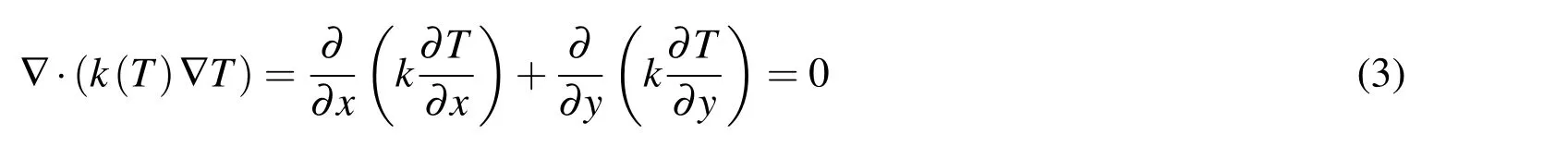
wherekis the temperature-dependent heat conduction coefficient andTis the temperature.There are several kinds of boundary conditions:

The inverse Cauchy problem is somewhat different from the standard boundary value problem.Overprescribed Cauchy data are given on part of the boundary,for example Dirichlet and Neumann boundary conditions or Dirichlet and Robin boundary conditions are both given on part of the boundary.Meanwhile,on the remaining part of boundary no information is given.Inverse Cauchy problems are known as an ill-posed system.To solve this ill-posed system numerically,a robust and sound solver is necessary to overcome the numerical instability.

It is worth to mention here that by using a new variable

Eq.(3)will be transformed into a Laplace equation while the boundary conditions in eqs.(4)-(5)are still linear with respect to the variableψand Eq.(6)will become nonlinear.This technique is known as the Kirchhoff transformation.After solving the boundary value problems of the new variableψ,the inverse Kirchhoff transformation is then adopted to obtain the solution for the physical quantityT.In this paper,we do not adopt the Kirchhoff transformation technique and keep the original partial differential equation system nonlinear.

2.2　Multiquadric radial basis functions

Assume the physical quantity we concern can be expressed by the radial basis functions as:

where xiis the position vector ofi-th observation point,sjis the position vector of thej-th source point,ˉris the radial distance between xiand sj,andcjis the undetermined coefficient.φis the radial basis function and in this paper the multiquadric radial basis function is selected as:

in whichcis a shape parameter and the value ofcis 1.5 throughout this paper.The value ofcinfluences the results of inverse Cauchy problems.However,if the value ofcis appropriate,the influence is not significant as mentioned later in example 1.The optimal selection ofcis not within the scope of this article and is left as an open problem.

More details of the multiquadric radial basis function can refer to[Hardy(1990)].Substituting the expression in eq.(8)into eq.(3)to eq.(6)for the inverse Cauchy problem,we will construct a system of nonlinear algebraic equations for unknown coefficientcj.Unfortunately this nonlinear algebraic equation system is ill-posed such that conventional numerical solvers fail due to the numerical instability.One can easily observe that the leading matrix for the radial basis functions is a full matrix which usually makes the ill-posed nature worse.

2.3　Residual norm based algorithm

The following derivation can be found in many related articles such as[Liu and Atluri(2012);Liu and Atluri(2011b)].Let us begin with a nonlinear algebraic system written as:

To solve this nonlinear algebraic equation system,an equivalent scalar equation can be written as

Let us construct a space-time manifold as:

where x0is the initial guess andQ(t)satisfies thatQ(t)>0,Q(0)=1,and it is a monotonically increasing function oftwithQ(∞)=∞.

In order to keep the trajectory of the solution x on the manifold,the following consistency equation should be satisfied:

whereλis the proportional constant.After some manipulations,the evolution equation of x can be found as

where v=Bu.Now let us consider the evolution of the residual vector as:

Substituting equation(15)into equation(16),it follows

Using the forward Euler scheme,we can discretize equation(17)as:

Now let us use the forward Euler scheme on equation(15),we can obtain the following equation

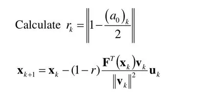
For a selected value ofr,we can rewrite equation(21)as an iteration formula[Liu and Atluri(2011b)]:

In the above equation,the relaxation parameter is used to make the iteration stabler.In a recent published paper[Liu(2013)],Liu further found the optimal value ofrneeds to satisfy the following relationship to guarantee the trajectory of x remain on the manifold:

2.4　Modified Tikhonov’s regularization method

The details of the following descriptions can be found in[Liu(2012)].Considering the following linear algebraic system as:

We use the following preconditioner written as:

and apply this preconditioner to equation(24)then we will obtain

with that B+B=In,i.e.,B+is the pseudo-inverse.

It is quite interesting to find that the regularized equation in equation(26)is very similar to that of the conventional Tikhonv’s regularization method.However,in equation(26)the regularization parameterˉαappears in the both sides of equation while for the conventional Tikhonov’s regularization method it appears only in the left-hand side.

Liu(2012)proposed that one can use equation(26)to formulate an iteration process as:

The convergence criterion of the iteration process for equation(27)can be set as:kup+1?upk≤?where?is a preselected small tolerance.Liu also provided a theoretical proof of the convergence as the following theorem states:

[Theorem 1]For Eq.(27)withˉα>0 the iterative sequence upconverges to the true solution utruemonotonically.

Although the convergence of the sequence is guaranteed,in computation reality to reach the final numerical convergence it may take too many steps such that it becomes not economic at all.It means that if one tries to find the solution of an ill-posed linear system,a lot of computation effort will be paid for the iteration process(equation(27))and sometimes it makes this iteration not economic at all.This algorithm needs to be further examined while it is used to solve the best direction u such that Bu-F=0.Since for each step in the iteration process stated in equation(22)for solving the nonlinear problem,this linear algebraic equation Bu-F=0 needs to be done if one tries to find the optimal direction.However,to find the solution of this linear problem may cost too many iteration steps for iteration process equation(27).Remember that we are not really interested in finding the best direction we only want to find an appropriate u such thata0is between 1 and 4.Therefore,we can check this criterion for each step of the inner iteration(equation(27))and terminate the inner iteration when the value ofa0is less than a prescribed critical valueac.Of course,it may still take too many steps to leta0being less than this prescribed critical valueacfor a severely ill-posed system.It is set that if the number of iteration steps for the inner loop exceeds a preselected maximum number Imax,we then stop the inner loop as well as the outer loop.It means that to find an appropriate direction of evolution using the proposed algorithm already becomes not economic and the whole process should be terminated.If the values ofacand Imaxare selected appropriately,the numerical results are acceptable as shown in the next section.

2.5　Double iteration process

Based on the abovementioned backgrounds,a double iteration process has been proposed[Yeih,Chan,Ku,Fan and Guan(2014)]and stated as the followings.

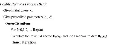
According to our numerical experiences,the value ofacis suggested to in the range from 2 to 4.Once the value ofacis less than 2,to seek the appropriate direction in the inner loop then consumes too many iteration steps.The value ofimaxactually depends on the selection ofac.If the value ofacis between 2 and 4,the value ofimaxis suggested to be in the range of 30,000 to 80,000 according to our numerical experiences.The selection ofεdepends on the system we want to solve.If the system is a well-posed system,the value ofεcan be very small such as 10?7.

(b) Ifp=Imax, terminates the whole process.

End of Inner Iteration

If RMSEe￡ or (b) is true then the outer iteration process stops; otherwise continue.

End of Outer Iteration Process.

However,if the system is an ill-posed system the value ofεshould not be very big and usually 10?3or 10?4is appropriate.It should be mentioned here that actually for an ill-posed system the value ofεcan be set as a small value for DIP since this tight convergence criterion cannot be reached and the whole DIP will be terminated due to the number of the inner iteration steps exceeds the maximum value Imax.It means the selection ofεis not critical at all.The value ofˉαneeds to be larger than the smallest eigenvalue of BTB which varies step by step.In calculation reality,a big enough value is selected.However,ifˉαis too big the iteration process for eq.(27)becomes slow.

3 Numerical examples

3.1　Example 1

After the weights of radial basis functions are obtained,a set of 313 uniformly distributed points and 41 boundary points are used to construct the temperature distribution contour.The value ofacis 2,the value ofˉαis 0.0001,the converge criterionε=0.001 and the maximum iteration steps for the inner loop Imax=30,000.The initial guesses for the unknown weights of the radial basis functions are all 0.01.

Figure 1:Distribution of source points for the radial basis functions in example 1.

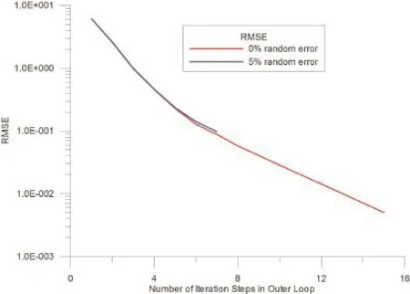
Figure 2:The root mean square errors versus the number of iteration steps for the outer loop in example 1.

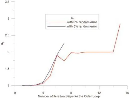
Figure 3:The profiles of a0 for both cases in example 1.

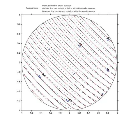
Figure 5:Comparisons between the exact solution and numerical solutions using 0%and 5%random error noise data.

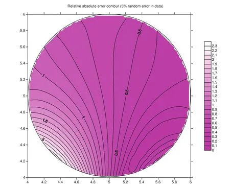
Figure 6:Relative absolute error contours for the case using 5%random error data.

In figure 2,the root mean square errors(RMSEs)for both cases are plotted with respect to the number of iteration steps for the outer loop.It can be observed that for both cases the RMSEs are not less than the convergence criterionε=0.001 before terminations.We further check the values ofa0for both cases as shown in figure 3.One can find that for the case using data without any noise the value ofa0exceeds the critical valueac=2 after 15 steps and for the case using data with maximum 5%absolute relative random errors the value ofa0exceeds the critical valueac=2 after 7 steps.It means that for both cases,the double iteration process terminates because searching for the appropriate direction becomes not economic.In figure 4,we examine the total accumulate iteration steps for the inner loops for both cases.It can be found that for both cases the final accumulated steps for the inner loop are less than 105steps.Since the most time-consuming step in the double iteration process occurs in the inner iteration loop,we can find that our proposed method indeed save computation efforts.Nevertheless,we still need to check whether or not the solution is acceptable.In figure 5,it can be seen that for the case using 0%error data the solution perfectly matches the exact solution while for the case using 5%absolute relative random error data the solution deviates from the exact solution a little bit.From figure 6,we can understand how the relative absolute error percentage distribution for the case using 5%absolute relative random error data is.It can be found the maximum absolute relative error percentage is about 2.4%.This result is quite good for the inverse Cauchy problem,especially the case we are studying now is nonlinear.Before closing this example,we use the parameters in this example and change the value of shape parametercfor the MQ radial basis functions and examine the maximum relative error for all representation points for eachc.The range ofcis from 0.5 to 20,and the increment incis 0.05.The absolute relative random error up to 5%is added in Cauchy data.The result is shown in figure 7 and one can see that within this range the maximum relative error for eachcis less than 12%.Actually,if the value ofcis less than 0.5,the maximum absolute relative error is very large(up to 300%or more).From this figure,one also can find that ifcis in this range the influence ofcis not significant.Therefore,in all cases studied in this article the value ofcis set as 1.5.

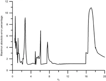
Figure 7:The maximum relative absolute error percentage for the case using 5%random error versus the shape parameter c.

3.2　Example 2

Two Cauchy problems are investigated here:for the first problem the Cauchy data are prescribed for the outer circle and no information is prescribed for the inner circle,for the second problem the Cauchy data are prescribed for the inner circle and no information is prescribed for the outer circle.For each Cauchy problem,the numerical solutions are obtained using data without any noise and data with maximum 5%relative absolute random errors.The value ofacis 3.5,the value ofˉαis 0.0001,the converge criterionε=0.0001 and the maximum iteration steps for the inner loop Imax=50,000.The initial guesses for the unknown weights of the radial basis functions are all 0.01.

The numerical results for both cases are illustrated in figures 9 and 10,respectively.It can be found that the numerical results using data without any noise are better than that using data with maximum 5%absolute relative random errors.Basically,no much difference can be found in both cases.The accuracies for both cases are very similar.The performances of the double iteration process are tabulated in table 1.The CPU times in this table represents the performances using Pentium?dualcore CPU E5200 at 2.50 GHz operating frequency.One can find out that due to the nonlinearity,as using data with maximum 5%absolute relative random error the maximum absolute relative error percentages are about 10%for both cases.In addition,from figures 8 and 9,one can find that the error tends to be larger near the boundary without information.Although the maximum relative error percentages for both cases are similar,it still can be told that using Cauchy data on the outer circle is better than using Cauchy data on the inner circle from the contour plots in figures 9 and 10.

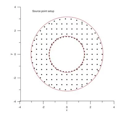
Figure 8:Source point setup for example 2.

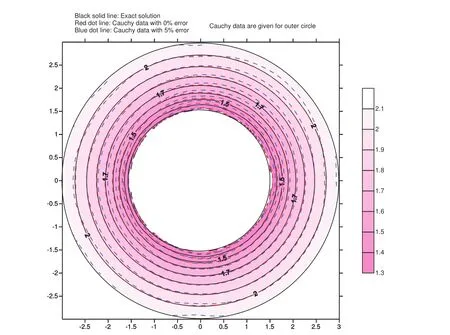
Figure 9:The temperature distribution for the Cauchy problem using data on the outer circle boundary.

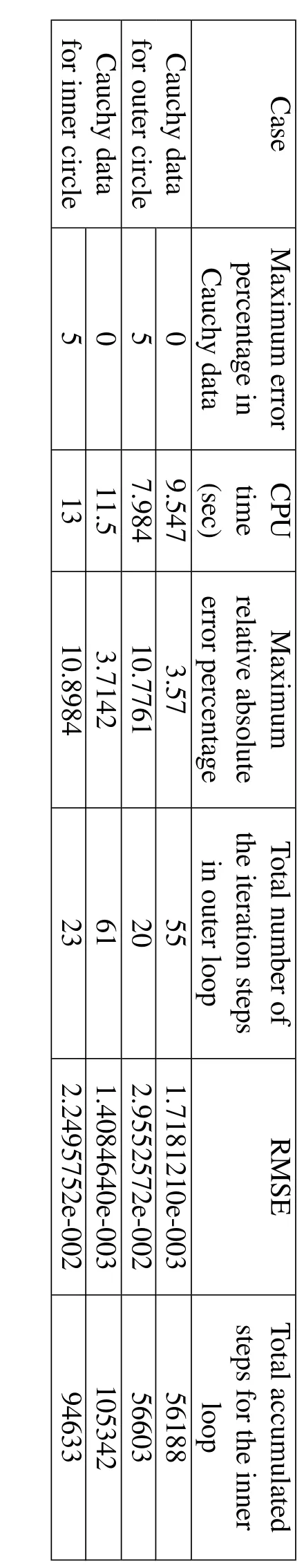
Table 1:Performance of double iteration process for example 2.

3.3　Example 3

In this example,a square region defined by{(x,y)|0≤x≤1;0≤y≤1}is considered.The temperature-dependent thermal conductivity isk(T)=exp(T).The temperature-dependent thermal conductivity now is nonlinear with respect to the temperature and it is very interesting to see what it will influence the numerical algorithm.The exact solution is designed as:T(x,y)=log(xy+5).Totally 100 points(25 points for each side and points are not placed at the corners)are arranged on the boundary and 169 uniformly distributed interior points accompanied with boundary points are used to be source points.After the weights are obtained,841 uniformly distributed interior points accompanied with boundary points are used to yield the temperature distribution.Cauchy data are given on the boundaries:y=0 andx=0.Two cases are examined:Cauchy data without any noise and Cauchy data with maximum 5%random relative absolute errors.The value ofacis 3.5,the value ofˉαis 0.001,the converge criterionε=0.0001 and the maximum iteration steps for the inner loop Imax=50,000.The initial guesses for the unknown weights of the radial basis functions are all 0.01.

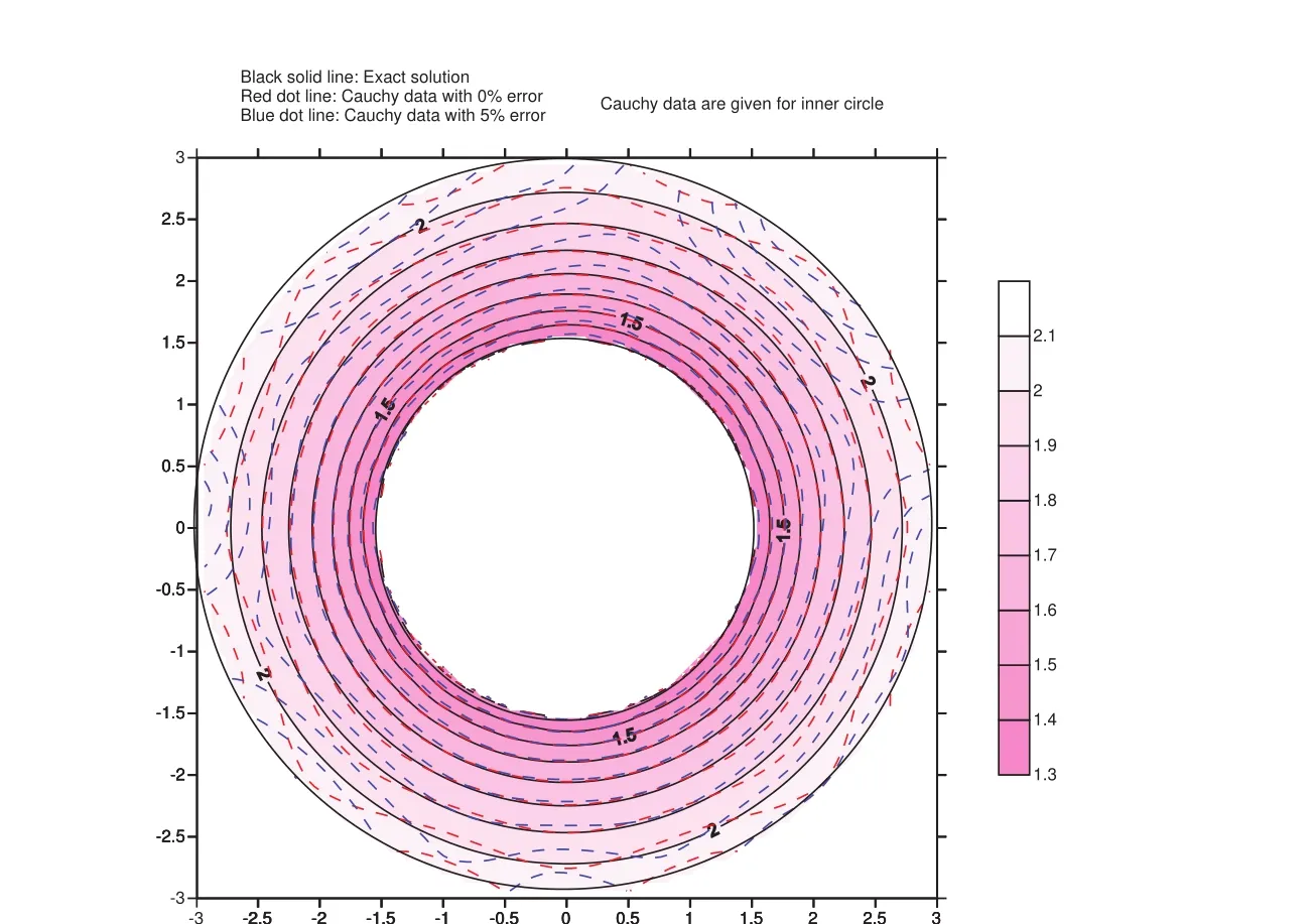
Figure 10:The temperature distribution for the Cauchy problem using data on the inner circle boundary.

The numerical solutions are illustrated in figure 11.Although it looks like that the temperature contour for the solution using Cauchy data with 5%random error seems not so close to the exact solution,the maximum absolute error percentage for all points is only 1.4677 percent.The reason why it looks so comes from that the difference between two adjacent contour lines is 0.01 which is very small.The computational CPU time for data without error is 20.063 sec and for data with maximum 5%absolute relative random error is 10.547 sec.The final RMSE for data without error is 0.0051742671 and for data with maximum 5%absolute relative random error is 0.019615273.Once again,one can see that for both cases they do not meet the convergence criterion for RMSE.However,after the process terminates the results are still acceptable.

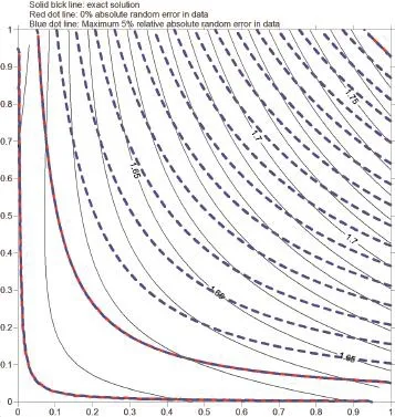
Figure 11:The temperature distribution for example 3.

3.4　Example 4

The result is sketched in figure 12.Compare this with figure 5,one can find out that using conventional Cauchy data seems better than using nonlinear Cauchy data(eq.(4)and eq.(6))under the same noise level.The reason should come from the nonlinearity which may enlarge the errors in data during calculation.

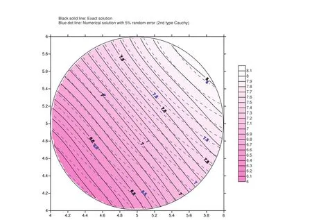
Figure 12:The temperature distribution for using Dirichlet and nonlinear Robin conditions as Cauchy data.

3.5　Example 5

The value ofacis 3.5,the value ofˉαis 0.001,the converge criterionε=0.05 and the maximum iteration steps for the inner loop Imax=80,000.The initial guesses for the unknown weights of the radial basis functions are all 0.01.

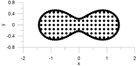
Figure 13:Source point setup for example 5.

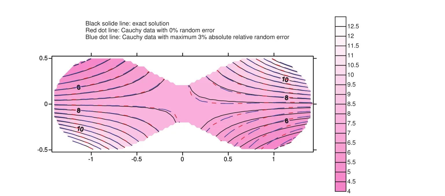
Figure 14:The temperature distributions for example 5.

The numerical results are shown in figure 14.It can be seen that the numerical results match the exact solution very well.The maximum absolute relative error percentage is less than 7 percent.

In this example,the DIP terminates due to the convergence criterionε=0.05 has been achieved for both cases with 0%and 5%maximum absolute relative random error in Cauchy data.

3.6　Example 6

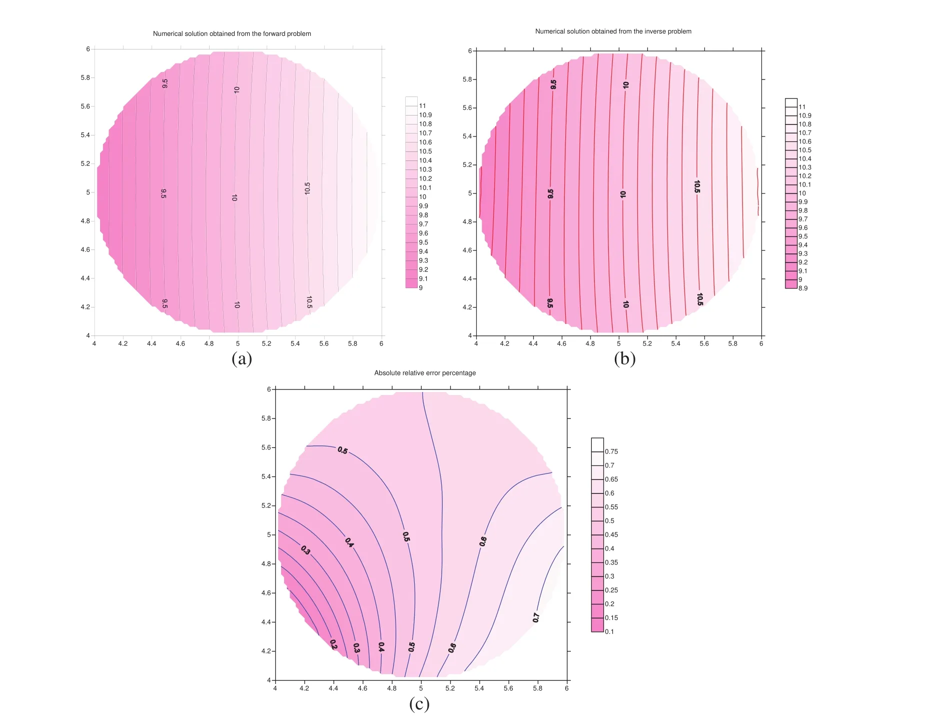
Figure 15:Numerical results:(a)Numerical solution for the forward problem;(b)numerical solution for the inverse Cauchy problem;(c)the absolute relative error percentage contour.

In the above five numerical examples,the numerical solutions are compared with analytical solutions.In real engineering problems,the so-called analytical solution may not exist.Therefore,the performance of DIP for inverse Cauchy problems without the analytical solution is quite interesting.In this example,the domain is a circular domain with radius equal to 1.The center of this circular domain is at(5,5).The parameters used are:ˉα=0.0001,ac=2.0,Imax=30000,ε=0.0001.The weights for the radial basis functions are set as 0.01 initially.The setup for boundary points,interior points and representation points are the same as that in example 1.

The forward problem is first studied.The Dirichlet data is given as:T(ˉθ)=10+cosˉθon the boundary whereˉθis the angle for the cylindrical coordinate system measuring from the center of the circular domain.The numerical solution for the forward problem is given in figure 15(a).

4 Conclusions

In this study,the double iteration process is used to deal with the Cauchy inverse problem of a nonlinear heat conduction equation.The double iteration process seeks for the appropriate evolution direction by using the MTRM for the inner loop.In order to avoid consuming too much computation time,once the direction satisfy the criteriona0

Bialecki,R.;Nowak,A.J.;(1981):Boundary value problems in heat conduction with nonlinear material and boundary conditions.Appl.Math.Modelling,vol.5,pp.416-21.

Cannon,J.R.(1967):Determination of the unknown coefficientk(u)in the equa-tion ?k(u)?u=0 from overspecified boundary data.Math.Anal.Appl.,vol.18,pp.112-14.

Chan,H.F.;Fan,C.M.(2013):The modified collocation Trefftz method and exponentially convergent scalar homotopy algorithm for the inverse boundary determination problem for the biharmonic equation.Journal of Mechanics,vol.29,pp.363-372.

Chan,H.F.;Fan,C.M.;Yeih,W.(2011):Solution of inverse boundary optimization problem by Trefftz method and exponentially convergent scalar homotopy algorithm.CMC:Computers,Materials,&Continua,vol.24,pp.125-142.

Gesele,G.;Linsmeier,J.;Drach,V.;Fricke,J.;Arens-Fischer,R.(1997):Temperature-dependent thermal conductivity of porous silicon.Journal of Physics D:Applied Physics,vol.30,no.21,p.2911.

Hansen,P.C.(1992):Analysis of discrete ill-posed problems by means of the L-curve.SIAM Rev.,vol.34,pp.561-580.

Hardy,R.L.(1990):Theory and applications of the multiquadric-biharmonic method.Computers and Mathematics with Applications,vol.19,no.8/9,pp.163–208,.

Hone,J.;Whitney,M.;Piskoti,C.;Zettl,A.(1999):Thermal conductivity of single-walled carbon nanotubes.Physical Review B,vol.59,no.4,pp.2514-2516.

Ingham,D.B.;Yuan,Y.(1993):The solution of a nonlinear inverse problem in heat transfer.IMA Journal of Applied Mathematics,vol.50,pp.113-132.

Ku,C.-Y.;Yeih,W.(2012):Dynamical Newton-like methods with adaptive stepsize for solving nonlinear algebraic equations.CMC:Computers,Materials,&Continua,vol.31,pp.173-200.

Ku,C.-Y.;Yeih,W.;Liu,C.-S.(2011):Dynamical Newton-like methods for solving ill-conditioned systems of nonlinear equations with applications to boundary value problems.CMES:Computer Modeling in Engineering&Sciences,vol.76,pp.83-108.

Landweber,L.(1951):An iteration formula for Fredholm integral equations of the first kind.Amer.J.Math,vol.73,pp.615–624.

Liu,C.-S.(2013):An Optimal Preconditioner with an Alternate Relaxation Parameter Used to Solve Ill-posed Linear Problems.CMES:Computer Modeling in Engineering&Sciences,vol.92,pp.241-269.

Liu,C.-S.(2012):Optimally generalized regularization methods for solving linear inverse problems.CMC:Computers,Materials,&Continua,vol.29,pp.103-127.

Liu,C.-S.;Atluri,S.N.(2008):A novel time integration method for solving a large system of non-linear algebraic equations.CMES:Computer Modeling inEngineering&Sciences,vol.31,pp.71-83.

Liu,C.-S.;Atluri,S.N.(2011a):An iterative algorithm for solving a system of nonlinear algebraic equations,F(x)=0,using the system of ODEs with an optimum in˙x=λ?αF+(1?α)BTF?;Bij=?Fi/?xj.CMES:Computer Modeling in Engineering&Sciences,vol.73,pp.395-431.

Liu,C.-S.;Atluri,S.N.(2011b):Simple"residual-norm"based algorithms,for the solution of a large system of non-linear algebraic equations,which converge faster than the Newton’s method.CMES:Computer Modeling in Engineering&Sciences,vol.71,pp.279-304.

Liu,C.-S.;Atluri,S.N.(2012):An iterative method using an optimal descent vector,for solving an ill-conditioned systemBX=b,better and faster than the conjugate gradient method.CMES:Computer Modeling in Engineering&Sciences,vol.80,pp.275-298.

Liu,C.-S;Kuo,C.-L.(2011):A dynamic Tikhonov regularization method for solving nonlinear ill-posed problems.CMES:Computer Modeling in Engineering&Sciences,vol.76,No.2,pp.109-132.

Mintsa,H.A.;Roy,G.;Nguyen,C.T.;Doucet,D.(2009):New temperature dependent thermal conductivity data for water-based nanofluids.International Journal of Thermal Sciences,vol.48,no.2,pp.367-371.

Morozov,V.A.(1966):On regularization of ill-posed problems and selection of regularization parameter.J.Comp.Math.Phys.,vol.6,pp.170-175.

Morozov,V.A.(1984):Methods forSolving Incorrectly Posed Problems.Springer,New York.

Tikhonov,A.N.;Arsenin,V.Y.(1977):Solution of Ill-posed Problems.Washington:Winston&Sons.

Tjalling,J.Y.(1955):Historical development of the Newton-Raphson method.SIAM Review,vol.37,pp.531–551.

Yeih,W.;Ku,C.-Y.;Liu,C.-S.;Chan,I.-Y.(2013):A scalar homotopy method with optimal hybrid search directions for solving nonlinear algebraic equations.CMES:Computer Modeling in Engineering&Sciences,vol.90,pp.255-282.

Yeih,W.;Chan,I.-Y.;Ku,C.-Y.;Fan,C.-M.;Guan,P.-C(2014):A double iteration process for solving the nonlinear algebraic equations,especially for illposed nonlinear algebraic equations.CMES:Computer Modeling in Engineering&Sciences,vol.99,no.2,pp.123-149.