Using Self-referencing Interlaced Submatrices to Determine the Number of Chemical Species in a Mixture

Miao Wang,Wan-ping Wang,Li-min Shao

Department of Chemistry,University of Science and Technology of China,Hefei 230026,China

Determining the number of chemical species is the first step in analyses of a chemical or biological system.A novel method is proposed to address this issue by taking advantage of frequency diflerences between chemical information and noise.Two interlaced submatrices were obtained by downsampling an original data spectra matrix in an interlacing manner.The two interlaced submatrices contained similar chemical information but diflerent noise levels.The number of relevant chemical species was determined through pairwise comparisons of principal components obtained by principal component analysis of the two interlaced submatrices.The proposed method,referred to as SRISM,uses two self-referencing interlaced submatrices to make the determination.SRISM was able to selectively distinguish relevant chemical species from various types of interference factors such as signal overlapping,minor components and noise in simulated datasets.Its performance was further validated using experimental datasets that contained high-levels of instrument aberrations,signal overlapping and collinearity.SRISM was also applied to infrared spectral data obtained from atmospheric monitoring.It has great potential for overcoming various types of interference factor.This method is mathematically rigorous,computationally efficient,and readily automated.

Key words:Number of chemical species,Bilinear two-way data matrix,Interlaced submatrix,Principal component analysis

I.INTRODUCTION

In mainstream analytical chemistry,experimental data formats have gradually changed from one-way vectors to two-way matrices.This change is due to,for the most part,advances in analytical instrumentation[1–5].Two-way data matrices contain a large amount of chemical information and,as such,pose a challenge to qualitative and quantitative analyses.Analyzing twoway experimental data matrices initially involves determining the number of chemical species in a chemical or biological system[6,7].Knowing the number of chemical species,one can then examine the intermediate species involved in chemical kinetics or identify impurities[8,9].For example,determining the number of chemical species permitted a more complete understanding of lithium battery dynamic following structural modification[10].In addition,knowing the correct number of chemical species enables self-modeling curve resolution to extract pure components from twoway data matrices without a prior knowledge of the mixture.For example,knowing the number of chemical species is necessary to determine the distribution of non-target chemical species in plant tissues[11].Determination of chemical species number makes possible the identification of interfacial phases of unknown polymeric materials[12].By comparison,complete resolutions using other analytical methods may largely depend on exhaustive iterations and expert interaction[13–16].

A variety of methods have been developed for determining the number of chemical species,and many of them are based on PCA[17].These methods can be classified into three categories:mathematical,empirical,and statistical[18].The first category includes such methods as orthogonal projection approach and least squares(OPALS)[19],ratio of eigenvalues calculated by smoothed principal component analysis and those calculated by ordinary principal component analysis(RESO)[20],and noise perturbation in functional principal component analysis(NPFPCA)[21].The second category includes such methods as factor indicator function(IND)[22],frequency analysis of eigenvectors(REFAE)[23],and morphological score(MS)[24].The third category includes such methods as Fisher variance ratio tests(F-test)[25,26],median absolute deviation(DRMAD)[27],and augmentation(DRAUG)[28].

These methods are eflective in some cases,but are rarely satisfactory for all data types.The application of multiple methods will likely yield a consensus of results.Many methods are more or less data-typespecific,which means satisfactory results are limited to a few types of data.Some methods include crucial parameters which require significant user intervention.As a result,such methods often yield ambiguous results.Mathematical methods are more robust when dealing with complex data matrices.Empirical indices assume an unsubstantiated noise distribution and statistical techniques are often limited by matrix size or normal noise distribution[29].For REFAE and MS methods,frequency analysis is employed to diflerentiate chemical information from noise.Frequency analysis reveals that chemical information is relatively low-frequency while noise frequency is high[24].With the attention to low-frequency chemical signals,RESO and NPFPCA can overcome,to some extent,the unwieldy problems of identifying minor components and heteroscedastic noise.

In this work,we propose a novel method,referred to as SRISM,in which two self-referencing interlaced submatrices play a key role.In SRISM,two submatrices are constructed respectively with odd and even column vectors chosen from the original data matrix in an interlacing manner.These are downsampled matrices that are obtained from the original one.The odd and even interlaced submatrices are similar with respect to low-frequency chemical information but are diflerent in terms of high-frequency noise.These two interlaced submatrices are decomposed into two sets of PCs using PCA.A pairwise comparison of the two sets of PCs readily yields the number of chemical species.SRISM was evaluated using both simulated and experimental datasets.The experimental data matrices were produced with up to six chemical species.Compared to other commonly used methods,SRISM was more robust when dealing with such interferences as signal overlapping,minor components,homoscedastic and heteroscedastic noise,instrument aberrations and collinearity.When applied to monitoring ammonia in infrared atmospheric spectra,it was able to detect ammonia in concentration of 0.1 ppm.Moreover,SRISM was shown to be mathematically rigorous,computationally efficient,and readily automated.

II.THEORY

Throughout this work,boldface lower-and uppercase letters denote vectors and matrices,respectively.All vectors are column vectors.The subscript is the matrix size.

Dm×ndenotes a bilinear two-way data matrix measured at fixed time intervals(m rows)and several diflerent wavenumbers(n columns).It contains chemical information and noise.According to sampling theory[28],low-frequency chemical information can be completely sampled when the Nyquist frequency is higher than the highest frequency of chemical information.Highfrequency noise is undersampled within various available sampling frequencies even when using the most advanced equipment.So Dm×nis downsampled by choosing all the s odd column vectors to form an odd interlaced submatrix,and the t remaining even column vectors are contained in an even interlaced submatrix,as shown in FIG.1.Based on a single experiment,andcontain similar completely sampled chemical information but diflerent undersampled noise.

PCA is broadly used to reduce the dimension of a data matrix by linearly combining the original variables that best account for the variance of the data matrix.When valid measurements are concerned,it seems reasonable that true data signals will be stronger than noise and thus contribute more to variance than the noise does.So it is possible to divide the primary from the secondary PCs.This is the premise of most methods based on PCA including ours.

The SRISM method comprises the following three steps(see FIG.1):

(i)Downsample Dm×nby choosing its column vectors in an interlacing manner,then constructwith the odd column vectors andwith the even column vectors.

(iii)Calculate the correlation coefficients between the paired PCs from PCoand PCe,then determine the number of chemical species with a 0.9 threshold.

It is noted that SRISM might yield overestimations if the data matrix contains large amount of low-frequency interferences,e.g.sloping baselines and strong fluorescent backgrounds in Raman spectra.In such cases,the original data should be preprocessed with baseline removal or background correction.

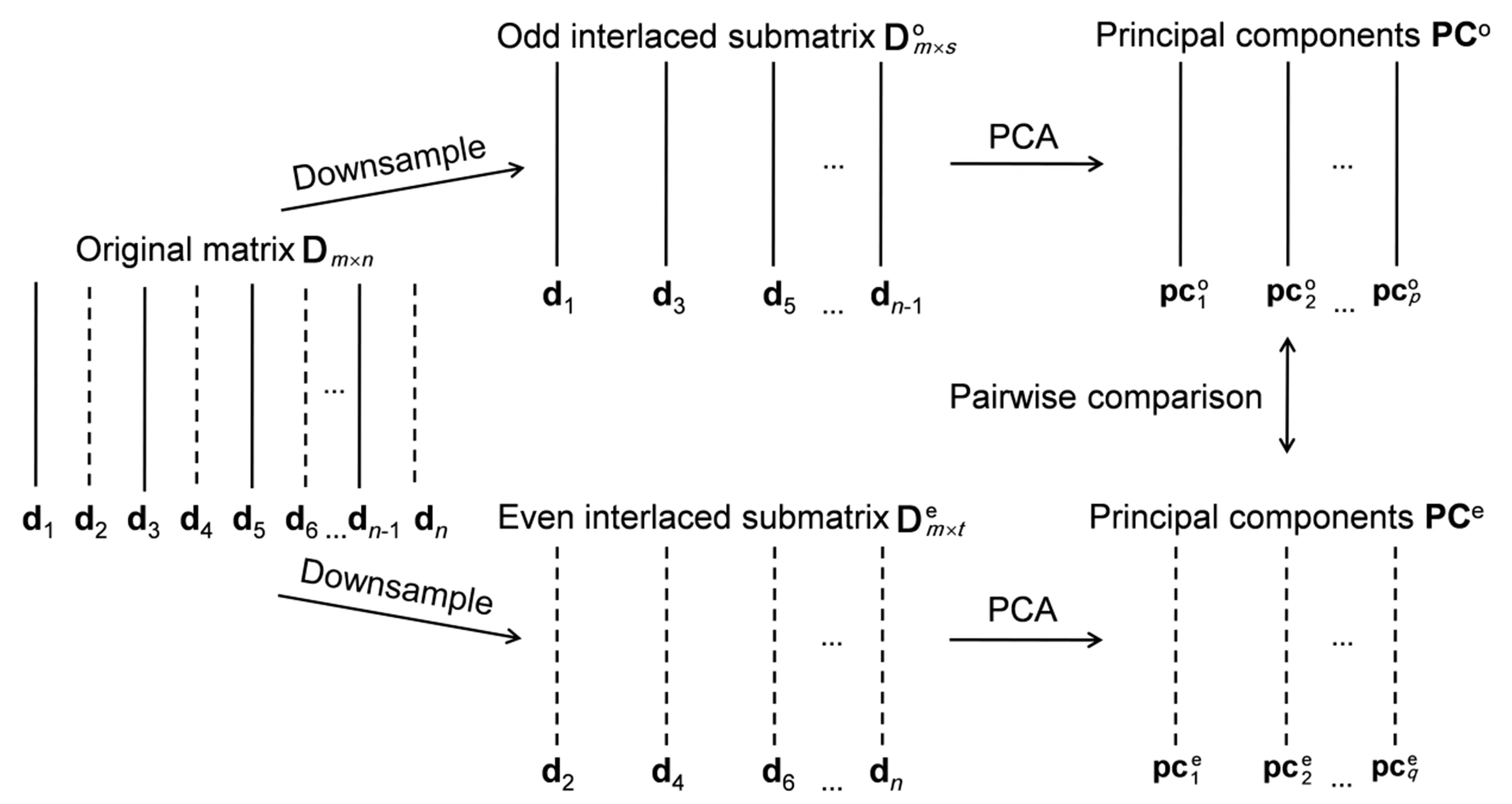
FIG.1 Steps using SRISM to determine the number of chemical species.d1,d2,d3,d4 ,d5,d6, ···,dn?1,dnare the column vectors of Dm×n.All the odd column vectors(d1,d3,d5,···,dn?1)form an odd interlaced submatrixand all the even column vectors(d2,d4 ,d6,···,dn)form an even interlaced submatrix.pc1o,pc2o,···,pcpo are the principal componentsof submatrix,and pc1e,pc2e,···,pcqeare theprincipal componentsof submatrix

III.EXPERIMENTAL METHODS

Theproposed SRISM method wasextensively evaluated using simulated gas chromatography coupled with infrared spectroscopy(GC-IR),experimental highperformance liquid chromatography coupled with diode array detector(HPLC-DAD),experimental pulsed field gradient nuclear magnetic resonance(NMR)datasets,and open-path Fourier transform infrared(OP/FT-IR)spectra obtained from atmospheric monitoring.All programs were written in MATLAB 2017a(The Math-Works,Inc.,Natick,MA).

A.Simulated datasets

Based on Beer’slaw,three-componentGC-IR datasets of diethyl ether,ammonia,and beta propiolactone were emulated with IR spectra and chromatograms.The IR spectra were within wavenumber range of 750?1250 cm?1(FIG.2(a)).The chromatograms were generated using a Gaussian function spanning a 10 min period(FIG.2(b)).The size of all simulated data matrices is 50-by-2075.

B.Experimental datasets

1.HPLC-DAD datasets

FIG.2(a)Spectra and(b)chromatograms of three chemical components used to simulate GC-IR data matrices.Dashed,black,and gray lines are spectra or chromatograms of diethyl ether,ammonia,and β-propiolactone,respectively.

Each rare-earth oxide (99.95%) was dissolved in hydrochloric acid solvent(1.0 mol/L)yielding a stock solution (1.000 g/L).A three-component mixturesolution contained Yb (2.0mg/L),Tm(2.0 mg/L),and Er(2.0 mg/L)(mixture 1).A sixcomponent mixture solution was prepared containing Lu(1.5 mg/L),Yb(1.0 mg/L),Tm(3.0 mg/L),Er(2.5 mg/L),Ho(3.8 mg/L),and Tb(2.1 mg/L)(mixture 2). Another six-component mixture solution contained Lu(1.0 mg/L),Yb(2.0 mg/L),Tm(3.5 mg/L),Er(3.2 mg/L),Ho(2.4 mg/L),and Tb(2.1 mg/L)(mixture 3). The three rare-earth mix-tures were analyzed with a FL 2000 HPLC Workstation(Spectra-Physics,USA)at multiple wavelengths of the Ultraviolet-visible(UV-Vis)spectroscopy detector(Spectra-Physics,USA)and 5 nm intervals.A 1-dodecanesulphonate solution(0.01 mol/L)was used as hydrophobic ion reagent to pretreat the reversed-phase column.Two mobile phase solutions were prepared containing 0.25 mol/L lactic acid(pH=2.5 and 4.5 respectively).A 0.0001 mol/L post-column reaction reagent of arsenazo III(Fluka Chemie,Switzerland)was prepared with redistilled water. All solutions were filtered through a 0.25μm membrane filter.The threecomponent rare-earth mixture 1 was eluted between the 4.5?9.9th min of a 15 min sampling duration at 0.344 s intervals,and was recorded within a 580?720 nm wavelength range as Dataset 1.The two six-component rare-earth mixtures 2 and 3 were detected between the 3.9?12.0th min of a 12 min sampling duration at 0.302 s intervals,and were recorded within wavelength ranges from 600 nm to 720 nm as Datasets 2 and 3,respectively.

2.Pulsed field gradient NMR datasets

A three-component mixture containing glucose(10.65 mg),sucrose(12.82 mg),and maltotriose(17.13 mg)was prepared in D2O(460μL)(mixture 4).A six-component mixture was produced containing methanol(3 μL),ethanol(4 μL),1-butanol(8 μL),sorbitol(15.59 mg),lysine(14.99 mg),and sucrose(21.13 mg)in D2O(460μL)(mixture 5).Pulsed field gradient experiments were performed at 25oC using a Bruker Avance 600 MHz spectrometer.The Bruker pulse sequence “ledbpgppr2s” was used with 0.20 s(mixture 4)and 0.18 s(mixture 5)diflusion delays and a net diflusion-encoding pulse width(δ)of 2 ms.Water signal was suppressed by presaturation.A spectral width of 20 ppm was used to produce 16000 complex data points with 8 scans for each gradient strength along with 8(mixture 4)and 4(mixture 5)dummy scans.An acquisition time of 1.36 s was used with a relaxation delay of 1.00 s.64000(mixture 4)and 32000(mixture 5)complex data points were Fourier transformed using an exponential window with a line broadening value of 1.0 Hz(mixture 4)and 0.3 Hz(mixture 5).For linear space in a nominal gradient,16 gradient strengths ranging between 1.465 and 47.865 G/cm were used for the three-component mixture 4.All compounds in mixture 4 have significant signals in the chemical shifts within the value of 6.000?2.8000 ppm designated as Dataset 4.32 gradient strengths ranging from 1.445 to 47.187 G/cm were collected for the sixcomponent mixture 5(Datasets 5?8,see Section IV).

3.OP/FT-IR datasets

OP/FT-IR spectra were measured around animal farms using two types of spectrometers(System A:Air-Sentry,Cerex Monitoring Solutions,Atlanta,GA and System B:MDA Corp.,Atlanta,GA).A Global source was coupled with an interferometer(Bomem Michelson 100,Canada),a splitter and a 25 cm expanding telescope.The expanded beam was reflected at a 100?200 m distance.The reflected beam was measured by a mercury-cadmium-teluride detector.Interferograms,with a resolution of 1 cm?1,were recorded continuously at an interval of several seconds.The interferograms were transformed to absorption spectra using 8 zero-filling factors and medium Norton-Beer function for apodization.The absorption spectra were then corrected through wavelet transformation to reduce the eflect of baseline shift. Absorption spectra with a wavenumber ranging from 750 cm?1to 1250 cm?1were used in our calculations.The spectra contained information that included both water and ammonia.Four datasets were collected over years as Datasets 9?12(see Table S1 in supplementary materials).

IV.RESULTS AND DISCUSSION

A.Three-component simulated datasets

All the GC-IR datasets were simulated with various levels of interference,such as signal overlapping,minor component,and noise.

1.Use of SRISM to determine the number of chemical species

Four GC-IR data matrices were simulated with 0.1%of homoscedastic noise added in four diflerent runs.The data matrices were analyzed by SRISM(FIG.3).In each case,the correlation coefficients were close to 1 for the first three PCs.SRISM analysis showed that the number of chemical species was 3 for each data matrix,which was the correct estimation of the chemical species number in the simulated dataset.

2.Eflects of chromatographic overlap,strength,and noise

Chromatographic overlap was simulated by moving the chromatographic peak of ammonia toward that of diethyl ether.Variations of chromatographic strength were simulated by decreasing the chromatographic peak height of ammonia.Homoscedastic or heteroscedastic noise was added to all data matrices.Corresponding data matrices were analyzed by SRISM and other commonly used methods.SRISM alone dealt well with the four types of interference of high levels and gave the correct number of chemical species(see Table I).

FIG.3 Correlation coefficients of paired PCs calculated from SRISM for four simulated GC-IR data matrices with 0.1%of homoscedastic noise added in four diflerent runs.The red lines mark the 0.9 threshold.

In Tables S2 and S3(see supplementary materials),it can be seen that mathematical methods generally produced an accurate number of chemical species.SRISM,OPALS,and DRAUG were able to detect the most overlapped or minor components.Empirical and statistical methods performed well when interference levels were low but they tended to underestimate numbers when interference levels were high.

The results shown in Tables S4 and S5(see supplementary materials)indicate that SRISM has a strong tolerance for the two types of noise present at each level and is able to correctly determine the number of chemical species.Most of other analytical methods were adversely aflected by high noise levels and tended to over-or under-estimate the number of chemical species.OPALS and MS were capable of successfully dealing with homoscedastic noise,but had more difficulty producing the correct number of chemical species in presence of heteroscedastic noise.This was also true with IND,DRMAD,and DRAUG.These methods were unable to deal with added levels of heteroscedastic noise because empirical IND and statistical DRMAD and DRAUG are based on the assumption that noise is specifically or normally distributed[17].By contrast,SRISM analysis depends upon frequency diflerences between chemical information and noise and,therefore,is free of such assumptions.Thus,it performs much better regardless of the noise type.Based on frequency diflerences,NPFPCA also estimated the correct number of chemical species in the presence of high-level noise.

B.Experimental datasets

FIG.S1(see supplementary materials)shows the three-dimensional(3D)plot and chromatograms of three HPLC-DAD Datasets 1?3.FIG.S1(a),(b)(see supplementary materials)show severe pump oscillations in the original Dataset 1 which consequently distorted chromatographic information. To reduce the severe instrument aberrations,chromatograms ranging 625?720 nm from the original Dataset 1 were used for later calculations.Pump oscillation was still present at a high level in Dataset 1.Dataset 1 size is 932-by-20.In FIG.S1(c,d)(see supplementary materials),highlevel instrument aberrations appeared in Datasets 2 and 3. Also present were high signal overlap levels(FIG.S1(c,d)in supplementary materials)in both Datasets 2 and 3 as evidenced by four distinct and one minor chromatographic peaks for the corresponding sixcomponent mixtures.The sizes of Datasets 2 and 3 are 1600-by-25.The numbers of chemical species for three HPLC-DAD Datasets 1,2,and 3 are 3,6,and 6,respectively.

Compared to spectra of GC-IR and HPLC-DAD,NMR spectra contain smaller high-frequency signals.Downsampling in decay-profile domain was carried out to avoid undersampling any of the chemical information.The three components mixture of glucose,sucrose,and maltotriose was detected and recorded as 10470-by-16 Dataset 4.The six-component mixture of methanol,ethanol,butanol,sorbitol,lysine,and sucrose was analyzed.The corresponding experimental NMR data matrix contained problematic noise and collinearity.To more easily analyze the six-component mixture,four data matrices were obtained using NMR spectral segments within chemical shift ranges of 3.280?3.240 ppm(262-by-32 Dataset 5,methonal response),2.000?1.149 ppm(5570-by-32 Dataset 6,butanol and lysine response),3.864?3.700 ppm(1074-by-32 Dataset 7,sucrose and sorbitol response)and 3.864?3.605 ppm(1696-by-32 Dataset 8,sucrose,sorbitol and lysine response).Therefore,the resulting chemical species number accounting for the five NMR Datasets 4,5,6,7,and 8 were 3,1,2,2,and 3,respectively.

1.Use of SRISM to determine the number of chemical species

The SRISM results for the experimental data matrices are shown in FIG.4.Eight plots demonstrate that the correlation coefficients of the first few paired PCs were close to 1 and higher than the 0.9 threshold.Correlation coefficients for the remaining PCs were all below threshold.The numbers of chemical species were determined to be 3,6,6,3,1,2,2,and 2,which are consistent with the actual numbers of chemical species except for Dataset 8.The SRISM results exhibit clear separation between the primary and secondary PCs.The remarkable diflerence between the two sets of PCs stems from their inherent frequency diflerences.SRISM was able to distinguish such diflerences to successfully separate the two types of PCs.In summary,this method pro-duced accurate numbers of chemical species in presence of high-level instrument aberrations,signal overlapping and collinearity.

TABLE I Numbers of chemical species determined by three categories of analysis methods using three-component simulated GC-IR datasetsawith various types of interference.

FIG.4 Correlation coefficients of paired PCs calculated from SRISM for eight experimental datasets.(a)?(c)HPLC-DAD datasets.(d)?(h)NMR datasets.The red lines mark the 0.9 threshold.

3D plots of the NMR experimental Datasets 4 and 8 are shown in FIG.S2(see supplementary materials).The high-level collinearity for the decay-profile made it more difficult to determine the number of chemical species especially for pulsed field gradient NMR spectra.The proposed SRISM method was able to successfully process multiple-component NMR datasets producing clear determination(FIG.4(d)?(g))with a high level of collinearity.FIG.4(h)illustrates that SRISM analysis showed a chemical species number of 2 for the threecomponent Dataset 8.Extremely similar decay-profilesfor sorbitol and lysine account for this incorrect estimation.

TABLE II Numbers of chemical species determined by three categories of methods for experimental HPLC-DAD and NMR datasets.

2.Comparison among three categories of methods

The eight experimental data matrices were also analyzed by several other commonly used methods to determine the number of relevant chemical species.The results(Table II)show that SRISM determined the correct number of chemical species for 7 out of 8 cases,achieving the highest accuracy for any of the analytical methods tested. SRISM appeared to perform well in the presence of high interference levels of low-frequency pump oscillation and signal overlapping in Datasets 1?3. These types of high-level interference were not adequately handled by other methods.SRSIM,NPFPCA and REFAE were able to deal with the high-level collinearity in the threecomponent Dataset 4,and the others cannot yield reliable results(see FIG.S3 in supplementary materials).Based on frequency diflerences,RESO,REFAE and MS performed well with some datasets,but tended to yield underestimations when dealing with complicated multiple-component datasets like those seen in Datasets 2 and 3.IND,F-test,DRMAD and DRAUG were reported to ofler surprisingly good results when noise levels have an assumed or normal distribution in other studies[17].However,they tended to overestimate the number of chemical species in the presence of instrument aberrations,signal overlapping and collinearity in the eight actual datasets.All methods failed for Dataset 8 in the presence of severe collinearity.

These methods were further evaluated in terms of calculation time.The results are listed in Table III.The size of data matrices varies from 932-by-20(Dataset 1)to 5570-by-32(Dataset 6).SRISM completed the calculation in a few milliseconds even for the largest Dataset 6.The calculation time of SRISM did not increase significantly with the size of dataset.SRISM was always one of the fastest methods based on the length of computational time listed in Table III.The other mathematical methods of analysis were more time-consuming for complex procedures.

3.Application of SRISM to infrared spectra of atmospheric monitoring

OP/FT-IR spectra were continuously measured in four sessions of atmospheric monitoring.The spectra within a wavenumber ranging 750?1250 cm?1feature information of water and ammonia.Water is always a significant component in air and produces strong infrared absorption[31].In order to detect ammonia during the monitoring session,10 groups of consecutive spectra were prepared and a matrix was constructed from each group to determine the chemical species number.We also used partial least square(PLS)to calculate the ammonia concentration of each spectrum.In FIG.5,the number of chemical species was determined by SRISM as 1 when the concentration of ammonia was lower than 0.1 ppm.When the ammonia levels exceeded 0.1 ppm,the number of chemical species determined by SRISM was considered to be 2.Taking water into consideration for both cases,the other chemical species detected was ammonia.In most cases,SRISM was sensitive to the presence of ammonia when concentrations were over 0.1 ppm.PLS provided reliable results when the concentration of ammonia was higher than 0.1 ppm,but had larger quantitative errors when dealing with spectra containing less ammonia[32].Therefore,SRISM is a useful tool for qualitatively atmospheric monitoring that provides a rapid response to the presence of ammonia without time-consuming calibration and is independent of established models.

TheOP/FT-IR Datasets9?12werealsoanalyzed in 10 groups of spectra by other methods(see Tables S6?S9 in supplementary materials).In real atmospheric monitoring data sets,there inevitably exist wind,dust and rain which consequently produce un-stable OP/FT-IR results and flawed data[33,34].In spite of the fact that Datasets 9?12 were measured under diflerent conditions and with diflerent instruments,SRISM yielded a correct number of chemical species in most cases.F-test showed similar efficacy for atmospheric monitoring and determined the chemical species number to be 3 for Dataset 9 containing high ammonia concentrations.By contrast,REFAE and MS underestimated the number of chemical species.Other methods tended to yield inconsistent chemical species numbers when the concentration of ammonia varied.Therefore,SRISM is a fast and powerful tool for atmospheric monitoring.

TABLE III Calculation timea(in unit of s)of three categories of methods used for analyzing experimental HPLC-DAD and NMR datasets.

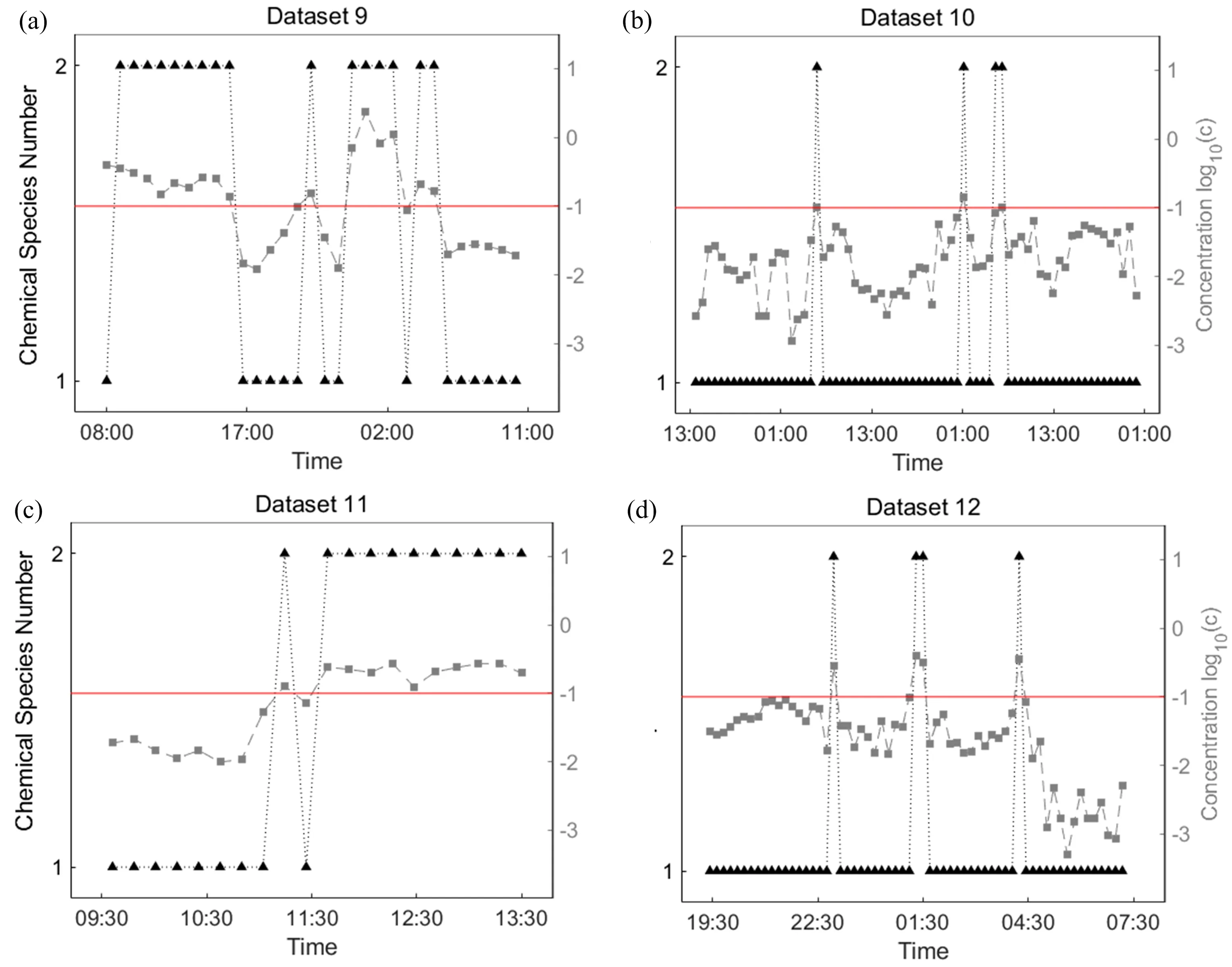
FIG.5 The number of chemical species in OP/FT-IR Datasets 9?12 determined by SRISM and concentration of ammonia calculated by PLS against time.The black dashed lines with triangle markers indicate chemical species number determined by SRISM.The dotted grey lines with square markers denote the maximum ammonia concentration(in unit of ppm)of 10 spectra calculated by PLS.The red lines denote the concentration of 0.1 ppm.The dotted grey lines and red lines are based on 10 logarithms of ammonia concentration for clarity.

V.CONCLUSION

In this report,the SRISM method is proposed as a mathematically rigorous,computationally efficient,and readily automated technique for determining the number of chemical species in a mixture.Its performance was evaluated using both simulated and experimental datasets.The results show that it tolerated various types of interferences such as signal overlapping,minor components,homoscedastic and heteroscedastic noise,instrument aberrations and collinearity to yield accurate results.SRISM utilizes frequency diflerences to diflerentiate between chemical information and noise.It has a large number of potential of application for various datasets,because chemical information is always completely sampled and noise is not.This method requires no user intervention to determine the number of chemical species,which makes it both objective and effi cient.Its reliable results are useful for qualitative and quantitative analyses of mixtures.

Supplementary materials:3D plots of experimental datasets,experimental chromatograms,and results of three categories of methods are available in FIGs.S1?S3 and Tables S1?S5.

VI.ACKNOWLEDGMENTS

This work was supported by the Program for Changjiang Scholars and Innovative Research Team in University and Fundamental Research Funds for the Central Universities(wk2060190040).The authors wish to express their thanks to Dr.Bin Yuan at Wuhan Institute of Physics and Mathematics,Chinese Academy of Sciences for providing the pulsed field gradient NMR data and in-depth discussions about the results.

[1]E.L.Schymanski,H.P.Singer,J.Slobodnik,I.M.Ipolyi,P.Oswald,M.Krauss,T.Schulze,P.Haglund,T.Letzel,S.Grosse,N.S.Thomaidis,A.Bletsou,C.Zwiener,M.Ib′a?nez,T.Portol′es,R.De Boer,M.J.Reid,M.Onghena,U.Kunkel,W.Schulz,A.Guillon,N.Noyon,G.Leroy,P.Bados,S.Bogialli,D.Stipaniˇcev,P.Rostkowski,and J.Hollender,Anal.Bioanal.Chem.407,21(2015).

[2]P.A.Mello,J.S.Barin,F.A.Duarte,C.A.Bizzi.L.O.Diehl,E.I.Muller,and E.M.M.Flores,Anal.Bioanal.Chem.405,24(2013).

[3]B.Meermann and M.Sperling,Anal.Bioanal.Chem.403,6(2012).

[4]M.Li,L.Yang,Y.Bai,and H.W.Liu,Anal.Chem.86,1(2013).

[5]S.Crotty,S.Geri?slioˇglu,K.J.Endres,C.Wesdemiotis,and U.S.Schubert,Anal.Chim.Acta 931,1(2016).

[6]Y.B.Monakhova and S.P.Mushtakova,Anal.Bioanal.Chem.409,13(2017).

[7]Y.B.Monakhova,S.P.Mushtakova,S.S.Kolesnikova,and S.A.Astakhov,Anal.Bioanal.Chem.397,3(2010).

[8]M.Garrido,F.X.Rius,and M.S.Larrechi,Anal.Bioanal.Chem.390,8(2008).

[9]N.D.Louren?co,J.A.Lopes,C.F.Almeida,M.C.Sarragu?ca,and H.M.Pinheiro,Anal.Bioanal.Chem.404,4(2012).

[10]P.Conti,S.Zamponi,M.Giorgetti,M.Berrettoni,and W.H.Smyrl,Anal.Chem.82,9(2010).

[11]J.B.Chen,S.Q.Sun,and Q.Zhou,Anal.Bioanal.Chem.407,19(2015).

[12]G.F.Trindade,M.L.Abel,C.Lowe,R.Tshulu,and J.F.Watts,Anal.Chem.90,6(2018).

[13]L.W.Hantao,H.G.Aleme,M.P.Pedroso,G.P.Sabin,R.J.Poppi,and F.Augusto,Anal.Chim.Acta 731,11(2012).

[14]H.Parastar,J.R.Radovi′c,J.M.Bayona,and R.Tauler,Anal.Bioanal.Chem.405,19(2013).

[15]Z.D.Zeng,H.M.Hugel,and P.J.Marriott,Anal.Bioanal.Chem.401,8(2011).

[16]A.Golshan,H.Abdollahi,S.Beyramysoltan,M.Maeder,K.Neymeyr,R.Rajko,and M.Sawall,R.Tauler,Anal.Chim.Acta 911,1(2016).

[17]E.R.Malinowski.Factor Analysis in Chemistry,3rd Edn.,New York:John Wiley&Sons(2002).

[18]W.Lu and L.M.Shao,J.Uni.Sci.Tech.China 44,11(2014).

[19]S.L.Hao and L.M.Shao,Chemom Intell Lab Syst.149,17(2015).

[20]Z.P.Chen,Y.Z.Liang,J.H.Jiang,Y.Li,J.Y.Qian,and R.Q.Yu,J.Chemom.13,1(1999).

[21]C.J.Xu,Y.Z.Liang,Y.Li,and Y.P.Du,Analyst 128,1(2003).

[22]E.R.Malinowski,Anal.Chem.49,4(1977).

[23]T.M.Rossi and I.M.Warner,Anal.Chem.58,4(1986).

[24]H.L.Shen,L.Stordrange,R.Manne,O.M.Kvalheim,and Y.Z.Liang,Chemom Intell Lab Syst.51,1(2000).

[25]E.R.Malinowski,J.Chemom.3,1(1989).

[26]E.R.Malinowski,J.Chemom.18,9(2004).

[27]E.R.Malinowski,J.Chemom.23,1(2009).

[28]E.R.Malinowski,J.Chemom.25,6(2011).

[29]N.M.Faber,L.M.C.Buydens,and G.Kateman,Anal.Chim.Acta 296,1(1994).

[30]J.G.Proakis,Digital Signal Processing:Principles,Algorithms,and Application,3rd Edn.,New York:Macmillan,(1996).

[31]P.R.Griffiths,L.M.Shao,and A.B.Leytem,Anal.Bioanal.Chem.393,1(2009).

[32]L.M.Shao,B.X.Liu,P.R.Griffiths,and A.B.Leytem,Appl.Spectrosc.65,7(2011).

[33]L.M.Shao and P.R.Griffiths,Anal.Chem.79,5(2007).

[34]L.M.Shao,C.W.Roske,and P.R.Griffiths,Anal.Bioanal.Chem.397,4(2010).