Keplerian Action,Convexity Optimization,and the 4-Body Problem

Kuo-Chang Chen

Department of Mathematics,National Tsing Hua University,Hsinchu,Taiwan

Abstract.In this paper we introduce a method to construct periodic solutions for the n-body problem with only boundary and topological constraints.Our approach is based on some novel features of the Keplerian action functional,constraint convex optimization techniques,and variational methods.We demonstrate the strength of this method by constructing relative periodic solutions for the planar four-body problem within a special topological class,and our results hold for an open set of masses.

Key Words:n-body problem,variational methods,periodic solutions,convex optimization.

1 Introduction

The Newtonian n-body body problem concerns the motion of n masses m1,···,mn≥0 moving in Rd,d∈{1,2,3},in accordance with Newton’s law of universal gravitation:

where xk∈Rdis the position of mk,x=(x1,···,xn),and

is the(self-)potential energy.Let

be the kinetic energy and L(x,˙x)=U(x)+K(˙x)be the Lagrangian.Eq.(1.1)are Euler-Lagrange equations for the action functional

The case A0,Twill be denoted by AT.Unless specified otherwise,throughout this paper a“solution”of(1.1)is referred to a“classical solution”of(1.1).

Analytic construction for periodic solutions of(1.1)is an old school,while variational approach has become a fashion since the discovery of the hip-hop orbit with four bodies[16]and the figure-8 orbit[15]with three bodies.Their idea of imposing symmetry constraints on solution curves was subsequently applied to many other examples,some notable successes been choreographic solutions[3,7,13,14,21,22,25,28,29],multiple choreographic solutions(such as the parallelogram four-body problem)[5–7],generalized hiphops[12,Section 4.2]and[30],and many other orbits with miscellaneous types of symmetries(such as symmetries with rotating circle property)[4,17–19].Most applications rely on manipulations of some equal masses.There are some examples without restriction on equal masses:the generalized hip-hops with the Italian symmetry[12,Section 4.2],some Hill type orbits[2],retrograde orbits for the three-body problem[9,10],and certain orbits with n-bodies extending Euler-Moulton relative equilibria[11].In some of these examples,simple order-two spatial symmetry were imposed without involving permutation of masses.Apart from them,to our knowledge there seems to be no substantial progress on variational constructions for periodic solutions of(1.1)with totally distinct masses.

Numerical experiments suggest that,however,many highly symmetric orbits with identical masses persist as one perturb the masses,with the only expense being the lose of some symmetry.The persistence is in fact observed in many examples for a fairly large range of masses.Some curious experiments on perturbing masses for orbits in[5]and[7,Section 5]are major incentives of our present work.Fig.1 is a very small list of motivating examples.With totally distinct masses,manipulations with symmetries are not helpful.Direct applications of global estimates in[9,10]are also not quite useful for n-body problems with n≥4,as to be explained later in this paper(Section 4).These solutions fall in certain topological families,and it is in general a difficult task to rigorously prove the existence of a real solution within a given topological family of curves.There must be some insights and artifices missing.

The purpose of this paper is to introduce a method to construct periodic solutions for the n-body problem with only boundary and topological constraints(Section 3).Our approach is based on some novel features of the Keplerian action functional(Section 2),some properties of the action functional(Section 4),and some constraint convex optimization techniques(Section 5).Our approach is a substantial improvement of methods in[9,10],and has no restriction on equal masses.We illustrate the strength of this method by constructing relative periodic solutions for the planar four-body problem within a special topological class(Section 6).

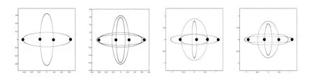
Figure 1:From left to right:The orbit in[5]with masses(m1,m2,m3,m4)=(1,1,1,1),a small perturbation with masses(0.8,0.9,1.1,1),and two large perturbation with masses(1,2,3,4)and(1,3,4,2).

2 The Kepler problem revisited

The Newtonian two-body problem,also called the Kepler problem,is one of the most classic problem in mechanics.Quoting Albouy[1],

“...the founding discoveries of Kepler and Newton remain strikingly beautiful,and indeed are so familiar to us that we sometimes forget that they contain surprising features.”

We revisit this ancient problem to explore some simple features of the Keplerian action functional that were not found in literature,but we find fascinating and useful in our applications.

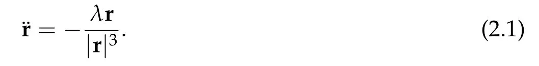
Consider the problem with masses m1,m2>0 and positions x1,x2∈R2.Let r=x2?x1be the relative position,λ>0 be the total mass multiplied by the gravitational constant,then the equation of motion is

A solution curve r(t)for the Kepler problem either traces out a conic with the origin as one of its foci,or composed of rectilinear motions with zero angular momentum.We shall identify the space containing the conic by R2or C and write r in polar form

For elliptical orbits(i.e.,e∈[0,1))and hyperbolic orbits(i.e.,e∈(1,∞)),the semi-latus rectum p,eccentricity e,and semi-major axis a are related by p=a(1?e2).The constant θ0is the phase angle between the major axis and the real line.

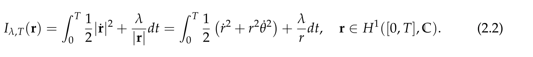
Eq.(2.1)is the Euler-Lagrange equation of the Keplerian action functional Iλ,Tdefined by This functional is well-known to be weakly lower semi-continuous[20],and is coercive(i.e.,Iλ,T(r)→∞as‖r‖H1→∞)on various subspaces.

From the perspective of the classical theory of variational calculus,one of the most natural and typical questions is to answer the minimization problem for the Keplerian action functional confined to the space

where boundary constraintsΩ0,Ω1are closed subsets of C.For various boundary constraints,coercivity of Iλ,Toften follows easily from simple variants of Poincar′e’s inequality.Typical examples are:one or both ofΩ0andΩ1are bounded,Ω0andΩ1are transversal lines,and so forth.Minimizers in such spaces are bound to exist.The question of our interest is therefore not about existence of minimizers,but about qualitative features of action minimizers and minimal action values.In particular,we would like to know whether or not minimizers fall inside the singular subspace;i.e.,the subset of curves with collisions.

The major purpose of this section is to analyze the minimization problem

for cases whereΩ0andΩ1are either singletons or rays emanating from the origin.The most critical property for our purpose is the Theorem 2.1 in Subsection 2.3 concerning convexity and monotonicity of infimum action values.

2.1 Minimization with two variable endpoints

The ray and line generated byξ/=0 are denoted respectively by

R+ξ={rξ:r∈[0,∞)}, Rξ={rξ:r∈R}.

For the special caseξ∈R,ξ>0,the ray it generates is simply the positive real axis R+.

Givenξ0,ξ1/= 0. The Keplerian action functional Iλ,Tattains its infimum on ΓT(R+ξ0,R+ξ1)if and only if the angleφ=∠ξ0ξ1between R+ξ0and R+ξ1is in(0,π](see[8,Proposition 1]for a more general statement and its proof).Union of such spaces and their singular subspaces can be characterized by

The symbol〈·,·〉stands for the standard scalar product in R2～=C.Clearly,minimization overΓT,φis the same as minimization overΓT(R+,R+eiφ).

The following proposition summarizes some discussions in[9,Section 5.1].

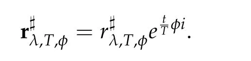
Proposition 2.1.Letφ∈(0,π],T>0,λ>0 be constants.Let

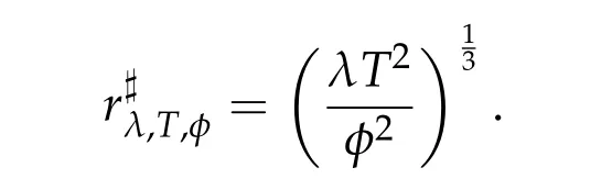
Then

OnΓT,φ,minimizers are congruent to

2.2 Minimization with two fixed endpoints

This term multiplied by the reduced mass m1m2/(m1+m2)is the more standard definition of total energy.

(i)A Lambert parameter is not constant on a family of arcs with the same configuration.

(ii)If f and g are two Lambert parameters,then|ξ0|+|ξ1|,|ξ0?ξ1|,f,and g are functionally dependent.

(iii)The energy h is a Lambert parameter.

There are several Lambert parameters identified in[1,Proposition 31].Apart from the transfer time,as identified by the classical Lambert theorem,what we need is just one:

Proposition 2.2(Albouy[1]).The action integral is a Lambert parameter.

In light of this,let us focus on rectilinear paths which begin and/or end with collision.For convenience we focus on paths ejecting from the origin at t=0 and moving along the positive real axis R+.Let Tλ(x0,x1,h)be the transfer time from x0to x1,0≤x0≤x1,without passing through collision,and with prescribed energy h.Let v1be the velocity of the path at time Tλ(x0,x1,h).Then by direct integration we have

where

When h<0,the second formula of Tλ(0,x,h)in(2.7b)represents the transfer time with non-monotonic rectilinear motion.In this case,in the first equation(2.7a)showing formula for Tλ(x0,x1,h),we shall use the first formula in(2.7b)for Tλ(0,x0,h).See the first graph in Fig.2 for a typical case–the graph of T1(0,2,h)as a function of h.

The energy h of the Keplerian action minimizer onΓT(0,ξ)with a prescribed transfer time T is implicitly given by formulae above.The minimum action value can be calculated accordingly via direct integration.For a monotonic rectilinear motion r ejecting from the origin at t=0,ending with position x>0,its action value is given by

Other cases can be easily derived from these formulae.

When a boundary constraint is a singleton,sayΩ0={ξ},we shall denote the space ΓT({ξ},Ω1)byΓT(ξ,Ω1)for simplicity,and likewise for other cases.Some special cases were summarized in the following proposition.

Proposition 2.3.Let T>0,λ>0 be constants,and let

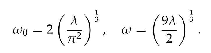
Then

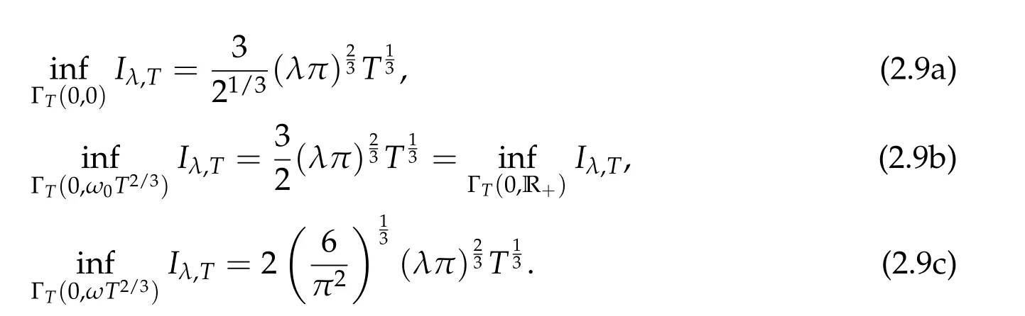
Proof.The second identity is achieved at the ejection orbit with zero velocity at the ending point,a case included in Proposition 2.1.It also minimizes Iλ,TonΓT(0,R+)since it is the unique monotonic ejection orbit along R+with zero velocity when t=T.The first identity is a simple corollary of the second.The third identity is the action value of the unique parabolic ejection orbit along the real line given by x(t)=ωt2/3.Details are simple calculations left to the reader.

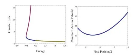
Figure 2:Left:Transfer time T1(0,2,h)versus energy h.Right:Half of action value of ejection Keplerian orbit with final position 2x and prescribed transfer time T=2.

2.3 Minimization with one fixed and one variable endpoint

Here we assume one fixed endpoint isξ/=0 and the other endpoint varies along a ray emanating from the origin.It is sufficient to consider minimization overΓT(ξ,R+)or,equivalently,ΓT(R+,ξ).Define the infimum Keplerian action Iλ,T:R+×[0,π]→R+by

Iλ,T(ρ,φ)=inf{Iλ,T(r):r∈ΓT(ρeiφ,R+)}.

Or equivalently,

Iλ,T(ρ,φ)=inf{Iλ,T(r):r∈ΓT(ρ,R+eiφ)}

=inf{Iλ,T(r):r∈ΓT(R+,ρeiφ)}.

Proposition 2.4.Givenξ/=0,letφ=Ar g(ξ).Consider the Keplerian action functional Iλ,Trestricted toΓT(R+,ξ).

(a)Ifφ∈[0,π/2],then for any action minimizer r of Iλ,T,r is free from collisions on[0,T]and˙r(0)⊥R+.

(b)Ifφ∈(π/2,π],then

Proof.The first part follows from a standard blow-up and deformation arguments(see for instances[8,Section 5],[18,Sections 7,9]and[31,Section 4.1]),outlined as follows.

Supposeφ∈[0,π/2).Let the deformation?y be given by

Then clearly?y∈Γ1(R+,y(1))has lower action value on[0,1]than y.Supposeφ=π/2.Given an arbitraryτ>1.Let?y be given by

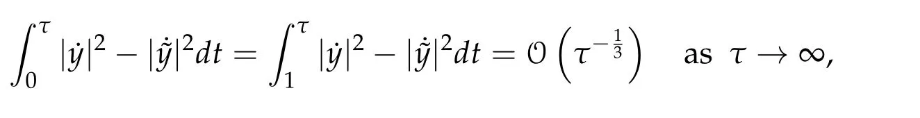
whereas

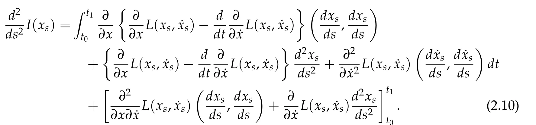
As a preparation for the main theorem in this subsection,we recall that in classical theory of variational calculus,the first and second variations for a functional of the form

are,assuming smoothness of the Lagrangian L,obtained by evaluating

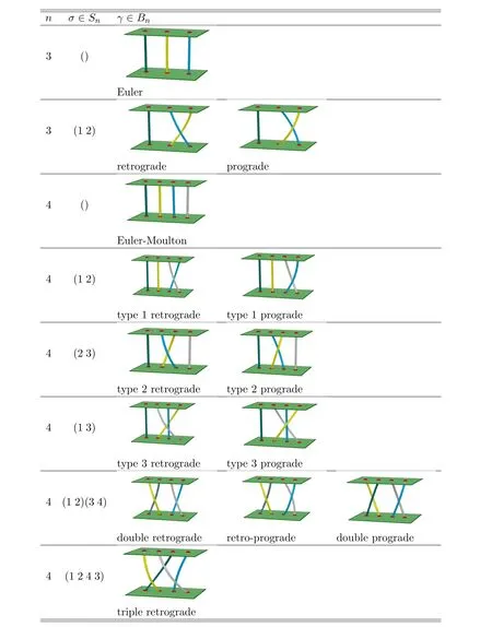
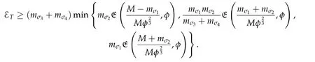
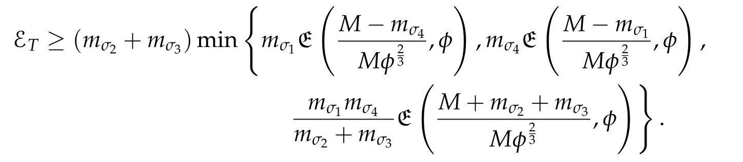
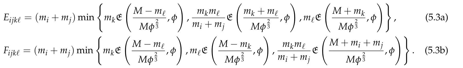
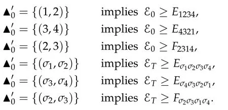
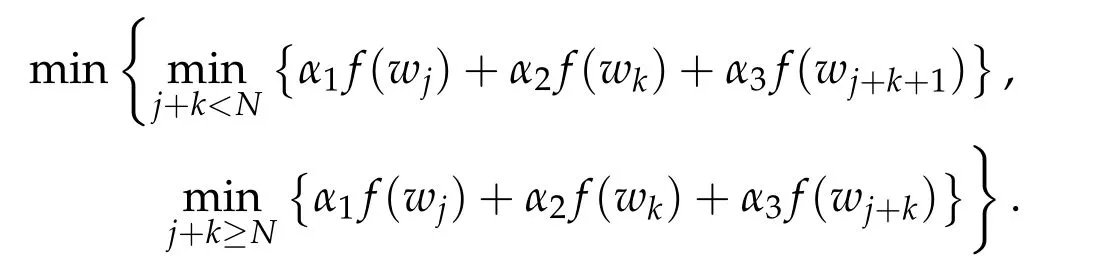
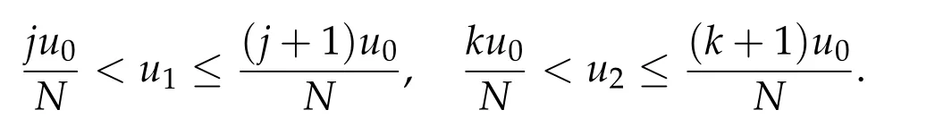
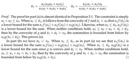
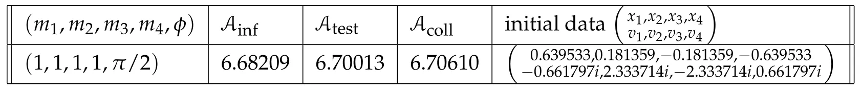
Second derivatives of the Lagrangian in above are bilinear forms on the space of admissible variations.One may replace the variation x+s h from x by a one-parameter family of curves{xs}?ε

Putting the second derivative in a more familiar form,via integration by parts,one has

Terms inside braces{·}vanish if the curve xshappens to be an extremal of the functional I.

In the second identity,the second term on the right-side equals zero because

due to the natural boundary condition,and

g(s)eiφ=rs(T)?r0(T)=s.

Figure 3:Graphs ofas a function ofρ.

By suitable scaling as did(2.3)we find

As a simple corollary of Theorem 2.1 and Proposition 2.4,we have

3 Algebraic and topological classifications of planar motions

Given n mass points moving on the complex plane.Consider the boundary constraints that all mass points are confined to move from one line L0to another line L1in a given time T.Without loss of generality we let L0be the real axis and let L1=R eφi,φ∈[0,π).The class of such paths is denoted by

Pφ,T,n:={x∈C([0,T],Cn):xk(0)∈R,e?iφxk(T)∈R,?k}.

Let?:={x∈Cn:xi=xjfor some i/=j}be the variety of collision configurations.The subset

3.1 Classification by the symmetric group Sn

By relabeling indices if necessary,we may confine our path space to only those which begin with a prescribed ordering.Givenσ∈Sn.Let

Example 3.3.The Figure-8 orbit[15]of the three-body problem passes across every collinear configuration but it is not action minimizing in our function space since it is never perpendicular to the line when its configuration turns collinear.

3.2 Classification by the braid group Bn

The braid group Bnon n strands generalizes the symmetric group Snon n symbols in the sense that Snis isomorphic to the quotient group Bn/Pn,where Pnis the normal subgroup of Bnconsisting of pure braids(i.e.,braids with the same starting and ending positions).Elements in Bnhave simple geometric interpretations that are ideal for descriptions of periodic planar n-body motions without collision,as the trajectory of mass points over one period in the three-dimensional space-time looks like a pure braid on n strands.In contrast,elements in Sn“forget”how these braids twist and wind,only keeping track of the final ordering.

Within any two braid classesγ0,γ1we may pick representatives c0inγ0,c1inγ1such that c0(T)=c1(0).The standard definition of braids multiplication

induces a well-defined multiplicationγ0·γ1and group structure for braid classes.The multiplicative identity is called the trivial braid class belonging to,which there is a Euler-Moulton’s relative equilibrium.The group of braid classes is exactly the braid group Bnon n strands.Due to its geometric nature,we refer the classification by Bna topological classification for planar motions.

Elementary braid types for the case of three bodies include trivial(Euler),retrograde,and prograde(direct)braids,for which we refer readers to[9,10]and references therein.Several elementary braids for the case of four bodies were listed in Fig.4.We exclude braids which are identical to some braids on the list after 180°rotation about the time axis.

4 The action functional for the n-body problem

In this section we provide some lower bound estimates for the action functional ATand show how they can be associated with certain constraint convex optimization problems.

Definition 4.1.Given x=(x1,···,xn)∈Pφ,T,n.Denote the relative position xi?xjby xij.We classify subscript pairs{(i,j):1≤i/=j≤n},(i,j)and(j,i)been considered equivalent,according to the behavior of xij=xi?xj:

For simplicity we use▲kto denote▲k(x)when the path x is fixed.We call elements in▲0colliding pairs,elements in▲1∪▲0,1order-preserving pairs,and elements in▲2∪▲0,2orderreversing pairs.The intersection▲0,1∩▲0,2is not necessarily empty since xijmay begin or end at 0.

Figure 4:Some elements of S n and Bn.

Here is the main theorem of this section.

where Aτand Bτ,τ∈{0,T},are given by

Therefore,given x∈Pφ,T,n,

Summing up,we find

By the homogeneity property(2.12)of EM,T(ρ,φ),we conclude that

The proof for

The rest of the proof for this case is the same as the caseτ=0.

With this estimate instead,one easily obtains

Now we briefly explain how Theorem 4.1 is associated with convex optimization problems and how it works for n-body problems.Details are to be carried out in later sections.

The main difficulty is to provide good lower bound estimates for the right-hand side;i.e.,action value of paths with collisions.

Then summations in Aτand Bτcan be expressed in termsσ.

Taking the standard ordered partition for subscript pairs and dropping terms involving E,the inequality(4.2)clearly implies

This is the lower bound estimate for the action functional one would obtained by following ideas in[9,10].However,this lower bound estimate is not sufficient to extend results in[9,10]to n-body problems with n≥4 and with general masses.

Theorem 4.1 is a very substantial improvement,especially when n≥4,since the contribution of summations involving E can be quite considerable.While estimating either Aτor Bτ,we wish to find a definite lower bound for summations involving E that is valid for all possible values of mutual distances|xij(τ)|,which are therefore treated as variables over which the summation is minimized.Apparently,mutual distances are not independent variables.Minimizing summations involving E with respect to mutual distances is a problem of convex optimization subject to constraints on the initial and final configurations.Simple techniques of convex analysis can be used to provide good lower bound estimates for this summation,as to be illustrated in the next section.

5 Some constraint convex optimization problems

Throughout this section we let f:R+→R+be a nonnegative convex function with a global minimum at u0>0.Consider the convex optimization problem of the form:

Here u=(u1,···,um)T.

A variant of this convex optimization problem considers an additional nonnegative convex function g:R+→R+with a global minimum at v0≤u0.The second type of optimization problem is of the form:

Here A u≤0 means each of its components is non-positive.

The optimization problem of the form(5.1)will be applied to estimation of Bτ,and(5.2)will be applied to estimation of Aτin Theorem 4.1.

5.1 The constraint convex optimization problem(5.1)

The propositions below provide examples of lower bound estimates for such constraint convex optimization problems.

Proposition 5.1.Consider the convex optimization problem(5.1)with m=3,A=(1,1,?1).Then

where

Proposition 5.2.Consider the convex optimization problem(5.1)with m=5.Supposeα1α4=α2α3.

(a)If

then

where

(b)If

then

where

Proof.By convexity,

Sinceα1α4=α2α3,the choice of A implies

Now we apply Propositions 5.1,5.2 to estimate B0in(4.2)for the four-body problem.

Proposition 5.3.Givenφ∈(0,π/2]and x∈Pφ,T,4.Suppose

x4(0)≤x3(0)≤x2(0)≤x1(0).

Then E0has lower bounds given as follows.

Proof.Fixφ∈(0,π/2]and let

Then

which has global minimum value 0 at u0=(M T2/φ2)1/3,by Corollary 2.1.

(u1,u2,u3,u4,u5)=(x13(0),x23(0),x14(0),x24(0),x34(0)),

(α1,α2,α3,α4,α5)=(m1m3,m2m3,m1m4,m2m4,m3m4).

(u1,u2,u3,u4,u5)=(x23(0),x24(0),x13(0),x14(0),x12(0)),

(α1,α2,α3,α4,α5)=(m2m3,m2m4,m1m3,m1m4,m1m2).

(u1,u2,u3,u4,u5)=(x12(0),x13(0),x24(0),x34(0),x14(0)),

(α1,α2,α3,α4,α5)=(m1m2,m1m3,m2m4,m3m4,m1m4).

We complete the proof.

The other two cases can be estimated by imitating the proof for Proposition 5.1.We skip details here because they are not used in our applications.

Similarly,one can obtain lower bound estimates for BTin(4.2):

Proposition 5.4.Givenφ∈(0,π/2],x∈Pφ,T,4,andσ∈S4.Suppose

Then EThas lower bounds given as follows.

For brevity,we introduce some notations to shorten expressions in Propositions 5.3 and 5.4.Given four positive masses(m1,m2,m3,m4)and a fixed angleφ∈(0,π/2].Let M be the total mass and let{i,j,k,?}={1,2,3,4}.Define

Note that Eijk?=Ejik?,Fijk?=Fjik?=Fij?k=Fji?k.Under assumptions of Propositions 5.3 and 5.4,these two propositions state that

We end this subsection with further improvements of Proposition 5.1,with which Propositions 5.2,5.3,5.4 can be improved accordingly.

Proposition 5.5.Consider the convex optimization problem(5.1)with m=3,A=(1,1,?1).Fix N≥3.Let

Proof.Given u1,u2>0,there exists some j,k∈{0,1,2,···}such that

By convexity of f and the assumption that f has minimum at u0>0,we always have

f(u1)≥f(wj), f(u2)≥f(wk).

If j+k

In either case,the right side can be written f(wj+k+1).Thus

α1f(u1)+α2f(u2)+α3f(u1+u2)≥α1f(wj)+α2f(wk)+α3f(wj+k+1).

If j+k≥N,then the convexity assumption on f ensures that

This implies the asserted inequality for the case j+k≥N.

5.2 The constraint convex optimization problem(5.2)with two convex functions

We only consider a few cases related to our applications.Arguments in here are similar to those in the previous subsection.We begin with some analogues of Proposition 5.1.

Proposition 5.6.Consider the convex optimization problem(5.2)with m=3,A=(1,1,?1).

(a)If?=2,then

where(

b)If?=1,then

where

Proposition 5.7.Consider the convex optimization problem(5.2)with m=3,?=2,A=(?1,1,1).Then

where

Now we apply Propositions 5.6,5.7 to estimate A0in(4.2)for the four-body problem.

Proposition 5.8.Givenφ∈(0,π/2]and x∈Pφ,T,4.Suppose

x4(0)≤x3(0)≤x2(0)≤x1(0).

Suppose 1≤i

Then by Corollary 2.1,

and f has global minimum value 0 at u0=(M T2)1/3φ?2/3,g has global minimum value 0 at v0=(M T2)1/3(π?φ)?2/3,which is less than or equal to u0.Note that xij(0)+xjk(0)=xik(0).

The lower bound in(a)is obtained by Proposition 5.6(b)with

The lower bound in(b)is obtained by Proposition 5.6(b)with

The lower bound in(c)is obtained by Proposition 5.7 with

The lower bound in(d)is obtained by Proposition 5.7 with

The lower bound in(e)is obtained by Proposition 5.1 with

Thus,we complete the proof.

Following the proof for Proposition 5.8,one immediately obtains the following estimate for BTin(4.2)by replacing xiby xσi.

Proposition 5.9.Givenφ∈(0,π/2],x∈Pφ,T,4,andσ∈S4.Suppose

Suppose 1≤i

6 Application to the four-body problem

Although we only focus on the four-body problem here,our estimates,which are based on Theorem 4.1 and properties of the Keplerian action functional,can be easily applied to general n-body problems.We wish that the application shown in this section will motivate many further applications.

If we are able to find a suitable collision-free test path in bσthat has even lower action value,then the inequality holds for an open set of masses and turning angles.

For the four-body problem,there are 6 pairs of(i,j)with i

In order to shorten our expressions,we fix positive masses(m1,m2,m3,m4),the turning angleφ,and use notations Eijk?,Fijk?,Gijk,Hijkdefined in(5.3),(5.4).Givenσ∈S4,1≤k

Here is our application to the four-body problem:

Theorem 6.1.Given T>0.Considerσ=(1243)and the triple retrograde braid bσas shown in Fig.4.There exist an open set M of positive masses(m1,m2,m3,m4)containing(1,1,1,1)and an open setΦof turning anglesφ∈(0,π/2]containingπ/2 such that there exist classical solutions for the four-body problem which minimizes the action functional on the component bσof bσ?Pφ,T,4.

where

{(1,3),(2,3),(2,4)}?▲1∪▲0,1, {(1,2),(1,4),(3,4)}?▲2∪▲0,2.

The table below lists the six possibilities and our selected ordered partitions for subscript pairs.

▲0▲′0▲′2(1,2)∈▲0{(1,2)}▲′1{(1,3),(2,3),(2,4)}{(1,4),(3,4)}(3,4)∈▲0{(3,4)}{(1,3),(2,3),(2,4)}{(1,2),(1,4)}(2,3)∈▲0{(2,3)}{(1,3),(2,4)}{(1,2),(1,4),(3,4)}(1,3)∈▲0{(1,3)}{(2,3),(2,4)}{(1,2),(1,4),(3,4)}={(σ3,σ4)}={(σ1,σ4),(σ1,σ2)}={(σ1,σ3),(σ2,σ3),(σ2,σ4)}(2,4)∈▲0{(2,4)}{(1,3),(2,3)}{(1,2),(1,4),(3,4)}={(σ1,σ2)}={(σ3,σ4),(σ1,σ4)}={(σ1,σ3),(σ2,σ3),(σ2,σ4)}(1,4)∈▲0{(1,4)}{(1,3),(2,3),(2,4)}{(1,2),(3,4)}={(σ2,σ3)}={(σ3,σ4),(σ1,σ4),(σ1,σ2)}={(σ1,σ3),(σ2,σ4)}

To estimate A0or ATin Theorem 4.1,we apply Proposition 5.8 for the first 3 cases,apply Proposition 5.9 for the last 3 cases.To estimate B0or BTin Theorem 4.1,we apply Proposition 5.3 for the first 3 cases,apply Proposition 5.4 for the last 3 cases.

In the first case,(1,2)∈▲0,A0is bounded from below by A12and B0is bounded from below by B12,where

Now,to complete the proof of the theorem,by continuity it is sufficient to prove that the inequality(6.2)holds for the special choice(m1,m2,m3,m4,φ)=(1,1,1,1,π/2)of masses and turning angle.We may just pick a suitable test path in bσfor this case and calculate its action value.For this case we have the following formula for E(ρ,φ):

The first line is simply the definition of E in(2.11).The second line holds because,for fixedρ,the minimizing Keplerian arc for I1,1(ρ,π/2)connects one end of the latus rectum to the pericentre,and by reflecting the arc with respect to the major axis we obtain a Keplerian arc connecting two ends of the latus rectum,which has length 2ρ.Since the action integral is a Lambert parameter(Proposition 2.2),the action value of this extended Keplerian arc is exactly the same as the rectilinear Keplerian arc ejecting from the origin and reaches 2ρat time 2,as they already have three Lambert parameters in common(using notations in Subsection 2.2,they are|ξ0|+|ξ1|,|ξ0?ξ1|,and transfer time).The action value of this extended Keplerian arc is therefore 2I1,1(ρ,π/2)=infΓ2(0,2ρ)I1,2,and the original minimizing Keplerian arc has half of this action.

Bearing this in mind,for our particular choice of masses and turning angle,we find the values of Aij’s and Bij’s are:

A12=A34=A23=A13=A24=A14≈13.4047,

B12=B34=B13=B24≈13.4122,

B23=B14≈13.4201.

Fix T=1/2.The test path selected is xtest=(x1,x2,x3,x4),where:

x1(t)=(0.6464 cos(πt)?0.0117 cos(3πt),?0.1824 sin(πt)?0.0035 sin(3πt)),

x2(t)=(0.1824 cos(πt)?0.0035 cos(3πt),0.6464 sin(πt)+0.0117 sin(3πt)),

x3(t)=?x2(t),

x4(t)=?x1(t).

Its action value,accurate to the fourth decimal place,is 6.7001,which is less than

This completes our proof.

Remark 6.1.We remark that the open sets M andΦdepends on the choice of braids,and the values of Aij’s and Bij’s are independent of the transfer time T.

It is often possible to find multiple ways of choosing lower bounds Aij,Bijfor Aτ,Bτby using Propositions 5.3,5.4,5.8,and 5.9.For example,in Theorem 6.1 we may choose

One may find all applicable combinations and choose the largest one.In fact,such lower bound estimates can be further improved using Proposition 5.5.In order to make it simple and clear,we do not pursuit for optimal bounds here.

Remark 6.2.In the proof we have used the fact that the action integral is a Lambert parameter to deduce

where x0=ρ(1?sinφ),x1=ρ(1+sinφ).The last equation can be calculated easily by using(2.8).

?

Acknowledgements

It is my great honor and pleasure to contribute in this special volume dedicated to Professor Paul Rabinowitz on his 80th birthday.Paul’s research work were great inspiration for my research interests,and his generous support and recognition have greatly influenced my research career.I also thank Jaeyoung Byeon,Yiming Long,and Zhi-Qiang Wang for their kind invitation to the Jeju meeting and this special issue.This work is supported in parts by the Ministry of Science and Technology in Taiwan.