High performance decoupled active and reactive power control for three-phase grid-tied inverters using model predictive control

Mohamed Azab

Abstract Finite control set-model predictive control (FCS-MPC) is employed in this paper to control the operation of a threephase grid-connected string inverter based on a direct PQ control scheme.The main objective is to achieve highperformance decoupled control of the active and reactive powers injected to the grid from distributed energy resources (DER).The FCS-MPC scheme instantaneously searches for and applies the optimum inverter switching state that can achieve certain goals, such as minimum deviation between reference and actual power; so that both power components (P and Q) are well controlled to their reference values.In addition, an effective method to attenuate undesired cross coupling between the P and Q control loops, which occurs only during transient operation, is investigated.The proposed method is based on the variation of the weight factors of the terms of the FCS-MPC cost function, so a higher weight factor is assigned to the cost function term that is exposed to greater disturbance.Empirical formulae of optimum weight factors as functions of the reference active and reactive power signals are proposed and mathematically derived.The investigated FCS-MPC control scheme is incorporated with the LVRT function to support the grid voltage in fulfilling and accomplishing the up-to-date grid codes.The LVRT algorithm is based on a modification of the references of active and reactive powers as functions of the instantaneous grid voltage such that suitable values of P and Q are injected to the grid during voltage sag.The performance of the elaborated FCS-MPC PQ scheme is studied under various operating scenarios, including steady-state and transient conditions.Results demonstrate the validity and effectiveness of the proposed scheme with regard to the achievement of high-performance operation and quick response of grid-tied inverters during normal and fault modes.

Keywords: Model predictive control, Finite control set, Grid-connected inverter, Active power,Reactive power,Distributed generation, Low voltage ride through, PQ theory, FCS-MPC, LVRT

1 Introduction

1.1 Literature review

A grid-connected inverter constitutes an essential part of modern DER (distributed energy resources) grid integration systems [1–10].During the last few years, many efforts have been made to ensure reliable operation of the grid-tied inverter by taking into consideration modern grid codes and standards [11–20].The increasing computation capability of high-speed digital signal processors (DSPs) and the availability of various hardwarein-the loop (HIL) control boards have facilitated the development and implementation of sophisticated control algorithms for achieving reliable grid-integrated systems[21–30].Accordingly, some new functions and features(such as LVRT) recommended by updated grid codes and standards can be added to the inverter control algorithm [19, 20, 23, 26–34].Such regulations obligate the grid-tied inverters to withstand unintentional grid voltage sag for a specific duration based on some LVRT profiles, which are customised in many countries [19, 20,31, 35–38].A modern control technique that has been utilised in recent years to control the operation of gridtied inverters is the FCS-MPC [39–55].Successful utilisation of the FCS-MPC algorithm has been reported in many studies [56–69].Most of the existing FCS-MPC schemes for grid-connected inverters are either current controlled [51, 61, 63, 66, 70, 71] or voltage controlled[72–75].

In current-controlled schemes, FCS-MPC regulates and controls as per the desired value the current injected to the grid from the DER by applying the adequate inverter switching state.In voltage-controlled schemes,FCS-MPC controls the inverter output voltage (voltage space vector), which indirectly controls the current injected to the grid.In this scheme, the computation of the voltage space vector is similar to the one used in the well-known SVM technique.

In this paper, FCS-MPC is employed to apply a direct PQ control strategy such that the active and reactive powers (P and Q) injected to the grid from the DER are directly controlled to their reference values; this is done through the application of the optimum inverter switching state to ensure a quick response.In recent years,considerable efforts have been made to overcome the major challenges of FCS-MPC that negatively affect its overall performance.One of these challenges is choosing the weight factors of the cost function.Thus, the topic of selecting the weight factors of the FCS-MPC cost function to optimise the scheme’s performance has gained much attention [41, 44, 46, 55, 76].Most of the weight factor determination methods are based on iterative range-sweeping techniques or evolutionary search algorithms because of the lack of theoretical design methodologies or analytical approaches for designing and adjusting these parameters.In general, all methods aim to assign a higher weight factor to a given objective term whenever it presents an unaccepted error [46].To achieve this task, the errors between the desired and actual values of the associated variables are usually used as inputs to the tuning algorithm [41,55,76].

Some methods assign discrete values to the weight factors (usually dual values) [41] or employ evolutionary search algorithms to determine the optimum weight factors involving the operating range [44], while other methods compute the dynamic weighting factor gain as functions of the errors such that the weight factors are tuned online [55, 76].Nevertheless, inappropriate dynamic weight factors can lead to the over-optimisation of the terms of the cost function.This deteriorates overall performance.Thus, there is a trade-off between simplicity and accuracy.To address such issues, this paper proposes an empirical weight factor-tuning method for achieving an optimised transient response of the overall FCS-MPC system.

1.2 Objective of the paper

The primary objective of the paper is to study and investigate an integrated control scheme for a three-phase grid-tied string inverter that can guarantee satisfactory steady-state performance as well as quick transient performance by employing decoupled control of the active and reactive powers (PQ) injected into the grid.The control scheme also attempts to consider the LVRT mode during grid voltage sag to satisfy the existing grid codes related to grid-connected inverters.The performance of the investigated scheme is studied under various operating conditions, including the normal and fault modes (grid voltage sag).Qualitative and quantitative analyses of steady state and transient responses are undertaken and addressed.Results demonstrate the validity and effectiveness of the discussed scheme in terms of the achievement of a high-performance three-phase grid integration system during both the normal and fault modes of operation.The rest of the paper is organized as follows.Section 2 provides an overview of the current-controlled FCS-MPC scheme for three-phase grid-tied inverters, and Section 3 details the different parts of the investigated system, including the computation of grid voltages and currents in (α-β) coordinates,the computation of power components (P and Q), the formulation of the cost function, and the adjustment of weight factors and also describes the LVRT mode.In Section 4, selected simulation results are presented and discussed, and qualitative and quantitative assessments on the results are also provided.Conclusions are drawn in Section 5, and the empirical formulae of variable weight factors and their mathematical derivations are presented in Additional file 1.

1.3 Main contribution

The main contributions of the paper are as follows:

(1) It proposes a simple and effective method of optimising the weighting factors of the FCS-MPC cost function for reducing undesired cross coupling between the P and Q control loops.Empirical formulae of optimum weight factors (as functions of active and reactive power references) are formulated and mathematically derived.

The proposed method varies the weight factors of the cost function only during detected transient periods and retains equal weight factors during steady-state operation.Thus, during steady-state operation, both terms of the cost function have the same levels of priority and contribution.However, during the transient period, the weight factors adjustment is governed by a simple, logical rule, i.e., granting a higher weight factor to the term that is exposed to higher undesired coupling until the error is restricted to predetermined satisfactory limits.

(2) It applies the concept of decoupled PQ control to incorporate LVRT capability, which is an essential option demanded by recently published grid codes (such as IEEE 1547, VDE-AR-N 4120 and IEC 62477–1).Most existing LVRT schemes are current-control based.They inject a suitable reactive current to the grid; consequently, reactive power is indirectly injected to the grid.However, in this paper, the LVRT is achieved through the direct injection of the optimum values of P and Q during a fault condition using the same FCS-MPC scheme; the corresponding reference powers (Pref&Qref) are instantaneously calculated within the FCS-MPC algorithm.

2 Current controlled FCS-MPC scheme for 3-Φ grid- connected string inverter

2.1 Single-line diagram and inverter power circuit

The single-line diagram of a typical three-phase PV grid integration system is illustrated in Fig.1.In this system,all PV arrays (considered as one of the DERs) are connected to a common DC bus of 600 V through the individual MPPT tracking units and suitable DC-DC converters incorporated with each PV array.The string inverter injects both active and reactive powers (P and Q) to the grid according to the mode of operation.The circuit diagram of a 3-Φ grid-connected inverter is shown in Fig.2; as shown, the energy produced from the distributed resource is injected to the grid through the inverter.A 3-Φ inductor LShaving a small equivalent series resistance RSis inserted at PCC between the inverter output and the grid [24].The voltage space vector UScan be described as a function of the DC link voltage and inverter switching states as follows:

Fig.1 Single line diagram of 3-Φ grid-tied String Inverter

Fig.2 Power Circuit of a 3-ΦGrid Connected String Inverter

where S1, S3and S5are the switching states of the upper power transistors of the inverter.The voltage space vector UScan be resolved into two orthogonal components(Uαand Uβ) in the (α-β reference frame, where their equivalent values are computed by:

The resultant components of inverter voltage space vector USfor all switching states are presented in Table 1.The six active inverter switching states and two nil switching states are used to control the operation of the grid-tied inverter in different configurations such as current-controlled mode or SPWM or SVM techniques.

Table 1 Switching States of a 3-Φ VSI Inverter

In FCS-MPC, the optimum inverter switching state is instantaneously selected and applied to the inverter to minimise a specific cost function; this is explained in the following sections.

2.2 Principle of current controlled FCS-MPC approach

In recent years, FCS-MPC has been adopted to control the operation of switching power converters such as grid-tied inverters [39–70, 76, 77].In the FCS-MPC technique, the future behaviour of the system is predicted for a finite time frame [40].Accordingly, the optimum future control action is applied to the system to satisfy a customised goal function [57–66], and the FCS-MPC algorithm is repeated at every sampling period [67–70, 76, 77].Generally, it is characterised by fast transient response and the ability to consider the nonlinearities and constraints in the control law [41–60].

Applying KVL to the circuit in Fig.2 yields:

The rates of change of grid currentsare rearranged:

Accordingly, (4.a) is employed to derive the instantaneous value of phase current iaat the (k+1)thsample as:

where TSis the sampling time, LSis the per-phase inductance of the inductor and RSis the equivalent series resistance of the inductor LS.

Similarly, the instantaneous grid currents of other phases,iband ic,at the (k+1)thsample are predicted as:

From (6.a), (6.b) and (6.c), the grid currents at the(k+1)thsample can be predicted through online measurement of the grid voltage (ean, ebn, ecn) and grid currents ia, iband icat the current kthsample.

The inverter output voltages (van, vbn, vcn) can be measured directly, while their (α-β) components in the stationary reference frame can be calculated based on (2.a)and (2.b).Unlike the hysteresis controllers or PI controllers driving PWM units, the FCS-MPC scheme instantaneously selects the optimum switching state every sampling period and achieves a specific goal function without requiring a PWM unit or hysteresis current controllers[40].

A simplified block diagram of a typical FCS-MPC scheme is presented in Fig.3, in which the predictive model block computes and predicts the grid currents at the (k+1)thsample for the eight inverter switching states.Inside the cost function computation block, a cost function is computed for all switching states.

The switching state that results in the minimum value of the cost function is considered as the optimum state to be applied.This task is performed inside the optimum switching state selection block shown in Fig.3.Consequently, if the reference grid currents,b andare given, the chosen cost function J, described by (7), is repeatedly evaluated during every sampling period for the eight possible switching states.One of them is the optimum switching state that results in the minimum value of the cost function at the (k+1)thsample.Accordingly, the actual grid current tracks the reference value with accepted error (deviation).

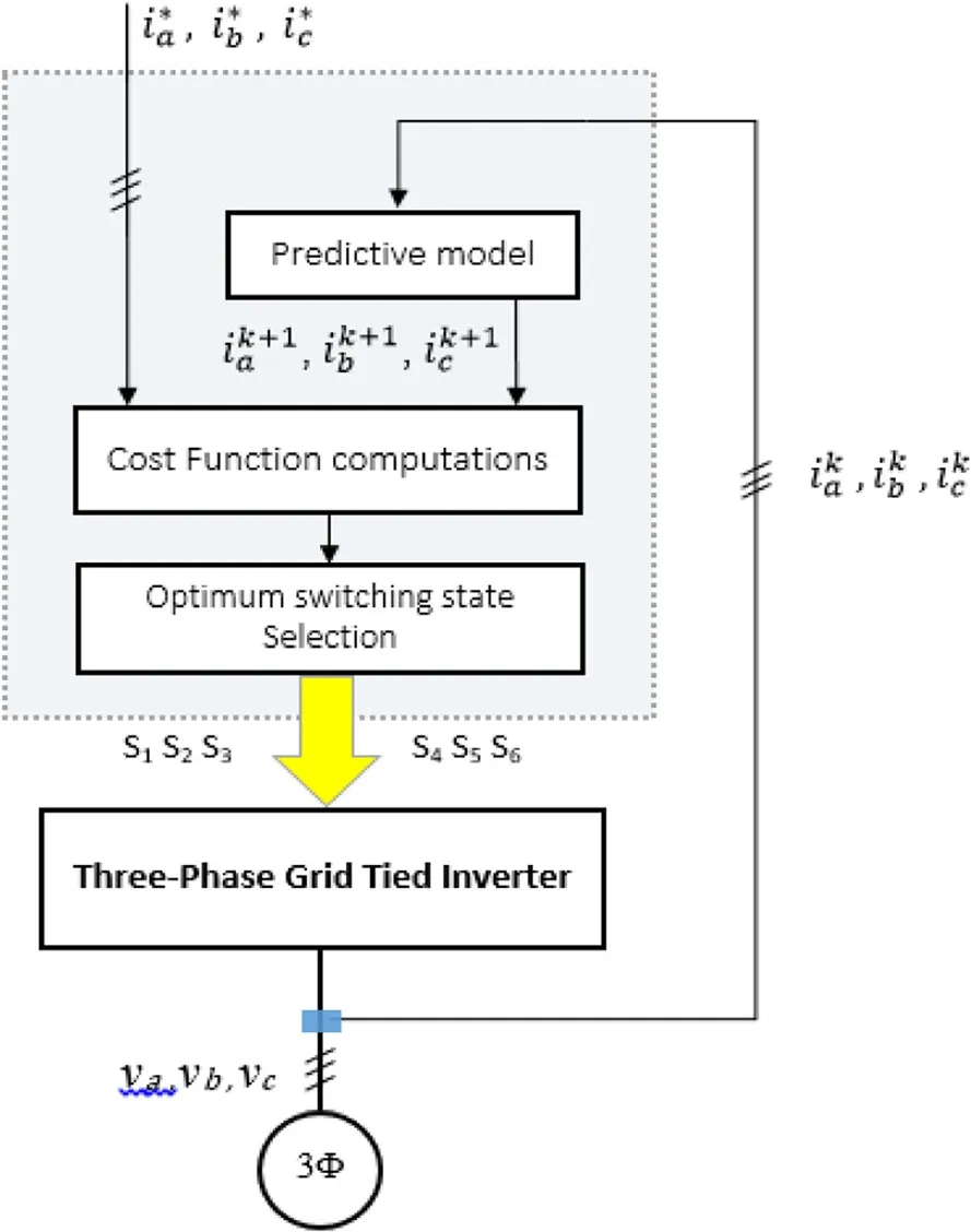
Fig.3 Simplified block diagrams of current controlled FCSMPC for grid-tied inverter

Excellent waveform tracking under FCS-MPC approach requires high sampling rates, which can be provided by high-speed data acquisition cards.

3 Description of the investigated decoupled PQ control system using FCS-MPC approach

The block diagram of the investigated FCS-MPC PQ system for a 3-Φ grid-connected string inverter is illustrated in Fig.4.The system is composed of two main blocks: (1) LVRT, which determines the mode of operation and computes the suitable reference signals of active and reactive powers; (2) The FCS-MPC system,which includes several blocks, such as prediction of grid currents and active and reactive powers, computation of cost function and selection of optimum switching state.All tasks are explained below in Subsections 3.1, 3.2 and 3.3.

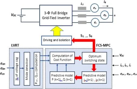
Fig.4 Block diagram of FCS-MPC scheme for three-phase grid-tied inverter

3.1 Computation of grid voltages and currents in (α-β)stationary reference frame

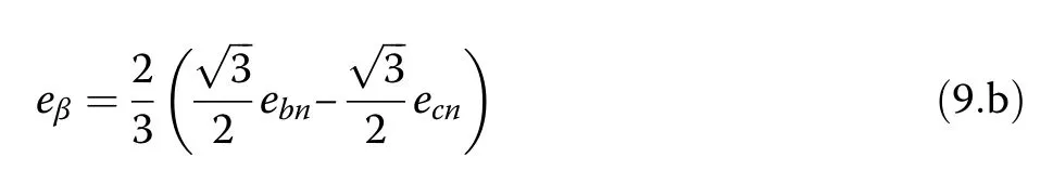
The (α-β) components of grid currents iαand iβare computed using (8.a) and (8.b), respectively.Similarly,the (α-β) components of grid voltages eαand eβare calculated using (9.a) and (9.b), respectively, based on the concept of the space vector as described by (1).Those components are essential in active and reactive power computations, as explained in Section 3.2.

3.2 Prediction of active and reactive power

The instantaneous active and reactive powers (P and Q)injected to the grid are computed as follows [21, 22, 78]:

Resolution of (6.a), (6.b) and (6.c) into the equivalent(α-β) components leads to the predicted iαand iβat the(k+1)thsample period as follows:

where uαand uβwere previously computed using (2)and tabulated in Table 1.eαand eβwere previously computed using (10).

From (8) to (11), the instantaneous active and reactive powers are predicted at the (k+1)thsample as follows[17]:

As the grid voltage has low variation compared to the sampling and switching frequencies, the grid voltage components eαand eβcan be considered constant during the sampling period, i.e.,

3.3 Formulation of cost function

The cost function is formulated to account for the active and reactive powers as follows:

where Prefand Qrefare the desired reference values of the active and reactive powers to be injected to the grid from the DER through the 3-Φ inverter.In (14), the first term of the objective function aims to minimise the active power deviation (ripple),while the second term aims to minimise the reactive power ripple, and both terms have the same degree of importance and make equal contribution.Accordingly,the instantaneous value of the cost function J in(14)is computed for all inverter switching states.The resultant values of the cost function are plotted in Fig.5 (a) for a small time frame of 70 μs (seven samples, each with a sampling period of 10 μs).From the results, applying inverter vectors U4and U5alternatively produces the minimum values of the cost function (J4and J5) during the selected time frame (in six samples out of seven) in conjunction with the null vectors U0or U7(in one sample out of seven).Thus,switching states 4 and 5 is the optimum selection (also see Fig.5 (b)).In addition, the null vector is considered as the optimum selected vector in one of the seven samples(at t=0.02005 s;J0is the minimum).Fig.5 (a) also shows that applying vectors U2and U3will yield the worst values of cost function(J2and J3)during the selected time frame.Similarly,applying vectors U1and U6will not result in an optimised cost function.Thus,vectors U2,U3,U1and U6are not used during the investigated time period.In Fig.5 (b), the overall minimum possible cost function Jmin(dotted line) is plotted together with J4and J5, which correspond to vectors U4and U5, respectively.In most FCS-MPC systems,weight factors are included in the terms of the cost function.Involving such weight factors allows the FCS-MPC system to assign a priority to the controlled variables on the design criteria.Thus,(14) is rewritten to involve weight factors in both terms of the cost function:

Fig.5 a Cost function for all possible inverter switching states.b Cost function when applying U4& U5 and the resultant minimum cost function as alteration between J4&J5

where wpand wqare the weight factors of active and reactive power terms, respectively.

3.4 Flowchart of the investigated FCS-MPC PQ control system

The flowchart of the FCS-MPC algorithm is shown in Fig.6(a);(2) and(11)–(15)are computed at each sample for all possible inverter switching states such that an optimum switching state is determined and applied during the next sample.

Initially, the system is investigated with constant weight factors (wp=wq=1) during the whole operation of the FCS-MPC system.

Then, those weight factors are varied during the transient periods, as explained in the flowchart of Fig.6 (b);this is described in detail in Additional file 1.

3.5 Adjustment of weight factors (Wp &Wq) of cost function

As shown in the flowchart presented in Fig.6 (b), the weight factors in (15) are adjusted based on a simple rule that imposes a penalty to the term causing cross coupling during the transient operation (by reducing its weight factor).

The same result can be obtained by granting higher priority or rewarding the negatively affected term of the cost function (by increasing its weight factor) during the transient periods.During steady-state operation, since no change occurs in the reference power, the weight factors are assigned to their initial values of unity.Once the algorithm detects a transient change in any of the reference signals (Prefor Qref), the weight factors are adjusted accordingly based on the rule summarised in Table 2 and previously illustrated in the flowchart of Fig.6(b).

As shown in Table 2, when the algorithm detects an abrupt change in Prefwhile Qrefhas no change (Sp >Sq), the weight factor wpis reduced to alleviate the disturbance that occurred on the Q loop from the P loop,while the weight factor wqis kept constant at unity.

Table 2 Selection criteria of weight factors

Similarly, when the algorithm detects an abrupt change in the Qrefsignal while Prefhas no change (Sq >Sp), the weight factor wpis kept constant at unity, while wqis reduced to alleviate the disturbance that occurred on the P loop from the Q loop.

This paper proposes a simple and effective method of tuning the weight factors (wpand wq).The details of the proposed method, including the mathematical derivation of the proposed formulae of wpand wq, are presented in Additional file 1.The optimum values of wpand wqare plotted in Fig.7(a) and (b), respectively.

Fig.7 Optimum values of weight factors of FCS-MPC cost function to minimize cross coupling during transient response.a.wp as a function of Pref. b. wq as a function of Qref

3.6 LVRT mode and modification of reference signals

The inverter control scheme is incorporated with an LVRT option to make it compatible with modern grid integration regulations and standards such as VDE-AR-N 4120, IEC 62477–1 and IEEE 1547[19,20,26,27,31,35–37].

In cases of fault and occurrence of voltage sag, the LVRT mode is enabled.Hence,the LVRT subroutine determines the level of voltage sag, and the reference power signals (Prefand Qref) are then computed such that the inverter injects a combination of active and reactive powers (or only reactive power) to the grid based on the actual value of the grid voltage sag (Vsag), as shown in Fig.6 (c).The flowchart of the LVRT subroutine illustrated in Fig.6 (c) demonstrates that the numerical value of the active and reactive powers to be injected to the grid is considered as a function of (Vsag).This relation is also presented as follows:

Fig.6 a Flowchart of the FCS-MPC algorithm.Flowchart of the overall elaborated FCS-MPC algorithm for 3-Φ grid connected string inverter.b Flowchart of weight factors adjustment.c Flowchart of LVRT algorithm

In (16), the voltage sag is discriminated in three zones:

Most developed countries have their own LVRT profiles, which the operation of modern grid-tied inverters should guarantee [23, 26,27,29,38].

4 Simulation results

The overall FCS-MPC system for a three-phase grid-tied string inverter was modelled and investigated in PSIM software?.The simulation parameters are summarised in Table 3.The simulation platform is PSIM and the sampling time is 20 μs (sampling rate is 50 kHz).In this section, the simulation results are categorised in three groups:

(1) Steady-state performance of the elaborated FCSMPC PQ system at normal operating conditions with quantitative assessment;

(2) Transient response of the FCS-MPC PQ system at normal operating conditions with quantitative assessment;

(3) Transient performance of LVRT under grid voltage sag.

4.1 Steady state performance

a.Unity PF Operation (Pref=10 kW, Qref=0 VAR)

The steady state performance of the investigated 3-Φ grid-tied inverter system was studied for unity PF operation.The reference active power was set to 10 kW, and the reference reactive power was zero.The instantaneous values of the resultant P and Q and the current injected to the grid are plotted in Figs.8 (a), (b) and (c),respectively.As the reference reactive power was zero,the current injected to the grid was in-phase with the grid voltage.The results shown in Figs.8 (a) and (b) indicate that both P and Q were well controlled to their desired values.The corresponding harmonic spectra of P, Q and the grid current are illustrated in Figs.9 (a), (b)and (c), respectively.

Fig.8 Steady state response of FCS-MPC at unity PF operation(Pref=10 kW, Qref=0 VAR).(a) Active power P; (b) Reactive power Q; (c) Grid phase voltage and current(Van&ia)

Fig.9 Harmonic spectra P, Q and ia injected to the grid at unity PF (Pref=10 kW, Qref=0 VAR).(a) Spectrum of the active power P;(b) Spectrum of the reactive power Q;(c) Spectrum of grid current(ia)

4.1.1 Quantitative analysis of steady state performance at unity PF

The quantitative analysis of steady state performance was conducted, and the results are presented in Table 4.The active power injected to the grid was 9.99 kW (desired reference value was 10 kW), while the reactive power was 68 VAR (desired reference value was zero VAR).

Table 3 Simulation parameters

However, it had negligible effect on the resultant PF(in this case, the actual PF was 0.999).Moreover, the computed THD of the grid current was 3.35%.

b.Zero PF Operation (Pref=0 W, Qref=10 kVAR)

The steady-state performance of the FCS-MPS-MPC was investigated for a different operating scenario: the reference active power was zero, while the reference reactive power was ?10 kVAR.The instantaneous values of the corresponding P, Q and the current injected to the grid are depicted in Fig.10 (a), (b) and (c), respectively.The results indicated that P and Q were controlled to their desired values.As the reference active power was zero (Zero PF), the grid current ialagged the grid voltage by 90°, as seen in Fig.10 (c).

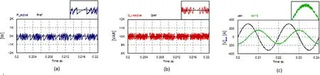
Fig.10 Steady state response of FCS-MPC at zero PF operation (Pref=0 W, Qref=10 kVAR).(a)Active power P;(b) Reactive power Q; (c) Grid phase voltage and current(Van&ia)

The corresponding harmonic spectra of P, Q and the grid current are depicted in Figs.11 (a), (b) and (c),respectively.

Fig.11 Harmonic spectra P,Q and ia injected to the grid at zero PF(Pref=0 W, Qref=10 kVAR).(a) Spectrum of the active power P;(b) Spectrum of the reactive power Q;(c) Spectrum of grid current(ia)

4.1.2 Quantitative analysis of steady state performance at zero PF

Quantitative analysis of the steady state performance was carried out, and the results are presented in Table 5.The reactive power injected to the grid was 10.005 kVAR, while the active power was ?100.6 W.Again, this only had a small effect on the resultant PF (in this case,the actual PF was 0.01).The computed THD of the grid current was 3.12%.

4.2 Transient performance

a.Step change of Pref(0 →10 kW) with Qref=0 VAR

The transient performance of the FCS-MPC system was investigated for different operating scenarios.In this subsection, the reference active power Prefhas a step change from 0 to 10 kW, while the reactive power reference Qrefis zero.

The transient responses were studied with fixed as well as adjustable weight factors, and the results are illustrated in Figs.12 and 13, respectively.

4.2.1 Quantitative analysis of step response of active power Pref(0 →10 kW) with Qref=0 VAR

A quantitative analysis was conducted of the transient response presented above, and the results are summarised in Table 6 for both FCS-MPC systems.

Table 4 Quantitative assessment of steady state performance at Unity PF (Pref=10 kW, Qref =0 VAR)

As shown in Fig.12(a), the active power with fixed weight factors had a fast transient response with a settling time of less than 2 ms (1.77 ms).Similarly, the observed settling time in the case of variable weight factors was also less than 2 ms (1.82 ms), as illustrated in Fig.13(a).

Fig.12 Transient response of FCS-MPC with fixed weight factors.(a)Active and reactive power.(b) Enlarged graph of reactive power.(c) weight factors; (d) Phase voltage and current

Fig.13 Transient response of FCS-MPC with variable weight factors.(a)Active and reactive power.(b) Enlarged graph of reactive power.(c) weight factors; (d) Phase voltage and current

In addition, both FCS-MPC schemes did not produce overshoot for the active power.

However, the reactive power component Q was negatively affected by the active power step change.The results indicated that the Q component was subjected to undesired cross coupling during the transient period in the case of the FCS-MPC scheme with fixed weight factors.This cross coupling on Q was approximately 1.6 kVAR and the time elapsed was 2 ms, as shown in Fig.12(b).

The results demonstrated that the proposed FCS-MPC scheme with variable weight factors effectively eliminates the cross coupling and successfully attenuates the disturbance to a negligible level during the transient period,as shown in Fig.13(a) and (b).

Figure 12(c) indicates that the weight factors were fixed to unity in the case of the fixed weight factors,while with variable weight factors, the weight factor wp(as depicted in.

Figure 13(c)) was changed according to the adjustment rule previously addressed in both Table 2 and Fig.7 (a).The grid currents sketched in Figs.12(d) and 13(d) indicate the successful operation of both schemes at unity PF during the transients.In addition, once the transient period had passed, both the fixed and variable weight factor schemes resulted in similar PF and THD of the current injected to the grid, as seen in Table 6.

b.Step change of Qref(0 →10 kVAR) with Pref=0 W

In this subsection, the transient performance of the FCS-MPC system is investigated in another operating scenario.The reference active power Prefwas set to zero,while the reactive power reference Qrefwas step changed from 0 to 10 kVAR.The transient responses were investigated with fixed as well as adjustable weight factors,and the results are illustrated in Figs.14 and 15,respectively.

4.2.2 Quantitative analysis of step response of reactive power Qref(0 →10 kVAR) with Pref=0 W

As shown in Fig.14(a), the reactive power with the FCS-MPC system of fixed weight factors had a fast transient response with a settling time of less than 2 ms (1.57 ms).

In the case of the FCS-MPC system with variable weight factors, the observed settling time was 0.42 ms (much less than the fixed weight factors case),as illustrated in Fig.15(a).

Both FCS-MPC schemes did not produce overshoot for the reactive power (as can be observed from Figs.14(a) and 15(a)).However, the FCS-MPC system with fixed weight factors slightly undershot before the reactive power settled down around the reference value,as illustrated in Fig.14(a).

In addition, the active power component P was negatively affected by the step change in the Q component.

The results indicated that the P component was subjected to severe undesired cross coupling during the transient period in the case of the fixed weight factors.The active power drop was approximately 2.7 kW, and it elapsed in 1.8 ms, as shown in Fig.14(b).

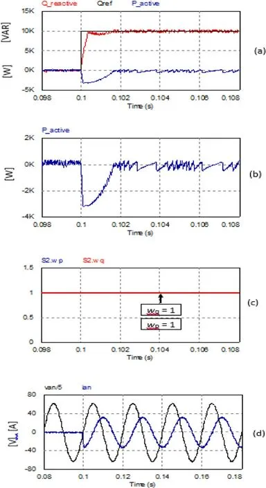
Fig.14 Transient response of FCS-MPC with fixed weight factors.(a)Active and reactive power.(b) Enlarged graph of reactive power.(c) weight factors.(d) Phase voltage and current

The results demonstrated that the proposed FCS-MPC scheme with variable weight factors effectively alleviates the cross coupling and successfully attenuates the disturbance to a negligible level during the transient period,as shown in Figs.15(a) and (b).

Figure 14(c) shows the unity weight factors for the fixed weight factors case, while in the case of variable weight factors, the weight factor wqwas changed, as depicted in Fig.15(c), according to the adjustment rule previously addressed in Table 2 and Fig.7 (b).

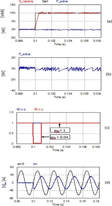
Fig.15 Transient response of FCS-MPC with variable weight factors.(a)Active and reactive power.(b) Enlarged graph of reactive power.(c) weight factors.(d) Phase voltage and current

The waveforms of the grid current sketched in Figs.14(d) and 15(d) indicate the successful operation of both schemes at zero PF during the transients.

Once the transient period had passed, both schemes(fixed and variable weight factors) resulted in similar PF and THD of the current injected to the grid, as seen in Table 7.

Table 5 Quantitative assessment of steady state performance at Zero PF(Pref=0 W, Qref=10 kVAR)

Table 6 Quantitative assessment of transient performance under step change of active power

Table 7 Quantitative assessment of transient performance under step change of reactive power

4.3 LVRT mode of the FCS-MPC system under grid voltage sag

The proposed FCS-MPC PQ control scheme is incorporated with an LVRT mode so that it withstands grid voltage sag for a short duration (determined by standard LVRT profiles) to be consistent with the upto-date grid code standards [27].

The operational scenario depends on the level of voltage sag, as explained in Section 3.6 and shown in the flowchart of Fig.6 (c).The first part of Section 4.3 presents an emulation of grid fault and voltage sag based on a standard LVRT profile.The LVRT profile is presented in Fig.16(a), and the corresponding grid voltage sag is plotted in Fig.16(b).

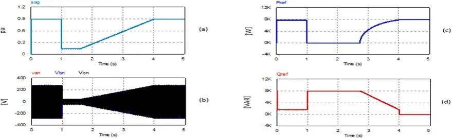
Fig.16 LVRT mode of FCS-MPC PQ control scheme

Consequently, the FCS-MPC PQ control unit generates the suitable reference active and reactive powers Prefand Qrefbased on (16), as illustrated in Figs.16(c) and (d), respectively.The second part of Section 4.3 illustrates the transient response of the FCS-MPC schemes under grid voltage sag.Figures 17 and 18 present the LVRT performance of the FCS-MPC PQ scheme with fixed and variable weight factors, respectively.Both groups of results prove that the FCS-MPC PQ scheme provides quick response and is able to enhance the LVRT capability of a grid-tied string inverter such that the LVRT option incorporated with the inverter control scheme is consistent with grid codes and standards.

5 Conclusion

In this paper, an FCS-MPC approach was used to control the operation of a three-phase grid-tied string inverter based on the concept of direct PQ control,providing a decoupled control of both active and reactive powers injected to the grid from the DER.

The cross-coupling problem associated with PQ control loops during transient operation was addressed and investigated, and an efficient method to minimise the undesired cross coupling between the P and Q control loops was proposed.The attenuation of cross coupling was achieved by varying the weight factors of the FCS-MPC cost function during the transient period.

The proposed method can be considered as a feedforward-tuning scheme for weight factors.In addition, the paper deduced empirical formulae to compute and tune the optimum weight factors as functions of reference active and reactive power signals.The relevant mathematical derivations were also presented.Results prove the validity and effectiveness of the proposed method with regard to the attenuation and alleviation of undesired cross coupling between the P and Q components.

The study involved both steady state and transient performances of the FCS-MPC scheme under variable operating scenarios, such as unity PF and zero PF operations.In addition, qualitative and quantitative analyses of the obtained results were carried out.

The elaborated FCS-MPC scheme inherently provided the LVRT mode, as requested by the updated grid codes and standards.The concept of a decoupled PQ control approach was applied to inject the necessary active and reactive powers to the grid during grid faults by modifying the instantaneous reference active and reactive powers based on the instantaneous grid voltage.

The results indicated that the adopted method was successful and able to support the LVRT capability of a grid-tied string inverter.

Fig.17 LVRT of FCS-MPC with fixed weight factors.a.Active power P.b.Reactive power Q.c.Grid current ia.d.steady state grid currents

Fig.18 LVRT of FCS-MPC with variable weight factors.a.Active power P.b.Reactive power Q.c.Grid current ia. d.steady state grid currents

The results demonstrate the capability of the FCSMPC approach in achieving a high-performance DER grid integration system that can be operated with different operating conditions, including fault mode

Abbreviations

ESR: Equivalent series resistance;DER: Distributed energy resources;DSP: Digital signal processor; FCS-MPC: Finite control set model predictive control; HIL: Hardware in the loop; KVL: Kirchhoff voltage law; MPC: Model predictive control; LVRT: Low voltage ride through;kW: Kilo Watt;PCC:Point of common coupling;PF: Power Factor; PI: Proportional integral controller;PLL: Phase locked loop; SVM:Space vector modulation; PV: Photovoltaic;PU: Per unit;Vsag:Per unit value of grid voltage sag; THD: Total harmonic distortion; VSI: Voltage source inverter; VAR:Volt-ampere reactive; 3-Φ: Three-Phase

6 Supplementary Information

The online version contains supplementary material available at https://doi.org/10.1186/s41601-021-00204-z.

Additional file 1.

Acknowledgements

The author is grateful to Mr.Bahaaeldin M.A.Moustafa, from Nile University(NU-Egypt) for his effort to download the needed references of the paper.The author is also grateful to Dr.Ali Abou-Sena, from Karlsruhe Institute of Technology (KIT-Germany) for his effort in revising the English language of this paper.

List of Symbols

VDCDC bus voltage

USInverter voltage space vector

eanGrid voltage of phase a

ebnGrid voltage of phase b

ecnGrid voltage of phase c

eαGrid voltage component of α-axis of (α?β)stationary reference frame

eβGrid voltage component of β-axis of(α?β) stationary reference frame

VanInverter o/p voltage of phase a

VbnInverter o/p voltage of phase b

VcnInverter o/p voltage of phase c

UαInverter o/p voltage component of α-axis of (α?β)stationary reference frame

UβInverter o/p voltage component of β-axis of(α?β)stationary reference frame

LSPer-phase grid filter inductor

RSPer-phase ESR of inductor LS

iagrid current of phase a

ibgrid current of phase b

icgrid current of phase c

iαGrid current component of α-axis of(α?β) stationary reference frame

iβGrid current component of β-axis of (α?β)stationary reference frame

TSSampling period of MPC algorithm

tdTime delay of reference signal

k Sample number k

i Switching state number (0 →6)

P Inst.value of active power injected to the grid

Q Inst.value of reactive power injected to the grid

Pk+1Predicted value of active power at sample (k+1)

PrefReference value of active power to be injected to grid

Qk+1Predicted value of reactive power at sample (k+1)

QrefReference value of reactive power to be injected to grid

J Cost function of FCS-MPC

JiCost function corresponding to switching state i

Ji(k+1) Cost function at the sample (k+1) corresponding to inverter switching state i

wp,wqWeight factors of MPC cost function

δpAbsolute error between reference and delayed reference active power signals

δqAbsolute error between reference and delayed reference reactive power signals

VsagPer unit value of grid voltage sag

Author’s contributions

The article has been prepared and edited by a single author “Mohamed Azab”who carried out all tasks of the article.English language revision has been carried out by a colleague from Karlsruhe Institute of Technology (KIT)and the final draft has been revised by a professional proofreading office“Paper True”.The author(s) read and approved the final manuscript.

Funding

This research did not receive any external funding.

Availability of data and materials

Not applicable.

Declarations

Competing interests

The authors declare that they have no known competing financial interests or personal relationships that could have appeared to influence the work reported in this paper.