
Prediction of boundary shear stress distribution in straight open channels using velocity distribution
2021-09-09 07:55BehzadMalvandiMahmoudMaghrebi
Water Science and Engineering 2021年2期
Behzad Malvandi,Mahmoud F.Maghrebi
Department of Civil Engineering,Ferdowsi University of Mashhad,Mashhad 91775-1111,Iran
Abstract Conventional methods for measuring local shear stress on the wetted perimeter of open channels are related to the measurement of the very low velocity close to the boundary.Measuring near-zero velocity values with high fluctuations has always been a difficult task for fluid flow near solid boundaries.To solve the observation problems,a new model was developed to estimate the distribution of boundary shear stress from the velocity distribution in open channels with different cross-sectional shapes.To estimate the shear stress at a point on the wetted perimeter by the model,the velocity must be measured at a point with a known normal distance to the boundary.The experimental work of some other researchers on channels with various cross-sectional shapes,including rectangular,trapezoidal,partially full circular,and compound shapes,was used to evaluate the performance of the proposed model.Optimized exponent coefficients for the model were found using the multivariate Newton method with the minimum of the mean absolute percentage error(MAPE)between the model and experimental data as the objective function.Subsequently,the calculated shear stress distributions along the wetted perimeter were compared with the experimental data.The most important advantage of the proposed model is its inherent simplicity.The mean MAPE value for the seven selected cross-sections was 6.9%.The best results were found in the cross-sections with less discontinuity of the wetted perimeter,including the compound,trapezoidal,and partially full circular pipes.In contrast,for the rectangular cross-section with an angle between the bed and walls of 90°,MAPE increased due to the large discontinuities.
Keywords:Open channel;Boundary shear stress;Viscous shear stress;Velocity distribution;Velocity gradient
1.Introduction
Determining the distribution of boundary shear stress in the vicinity of bed and banks of natural channels is a task fundamental to solving various problems in river morphology and flow restoration.These problems include determination of the rates of lateral erosion in rivers,sediment transport in shallow natural channels,and exact relationships between water depth and discharge in small river flows(Kean et al.,2009).To study the hydrodynamic forces acting on sediments,it is necessary to estimate bed shear stress(τ0)or shear velocity(u*)(Pope et al.,2006).Additionally,determining boundary shear stress is crucial in estimating cavitation.It can help river engineers predict river shape;protect river beds,banks,and flood control structures(Zarrati et al.,2008);and employ numerical methods.It is therefore important to calculate the resistance coefficients in rivers.Resistance coefficients usually utilize the law of resistance in twodimensional(2D)or three-dimensional(3D)flow calculations,which is related to the prediction of local bed shear stress(Tominaga and Sakaki,2010).Furthermore,knowledge of shear stress distribution can assist river engineers in estimating the shapes and dimensions of stable channels(Gholami et al.,2019).The boundary shear stress distribution is mainly related to the cross-sectional shape and the formation of secondary flows that exist on the plane perpendicular to the flow direction(Jin et al.,2004;Blanckaert et al.,2010).
Measurement of bed shear stress using a shear plate or cell is difficult and requires precise calibration and such measurements are only appropriate for some laboratory studies(Graham et al.,1992;Rankin and Hires,2000).In addition,when bed sediments begin to erode with different sediment levels,they produce unsatisfactory results(Pope et al.,2006).These procedures cannot be applied in rivers.Therefore,boundary shear stress can be determined from the observations of flow velocity or geometry,and the relationships of these values with boundary shear stress(Wilcock,1996).
Many analytical or semi-analytical methods have been proposed to calculate shear stress distribution(Shiono and Knight,1991;Zheng and Jin,1998;Jin et al.,2004;Yang and McCorquodale,2004;Yang,2005;Tang and Knight,2008)and to estimate mean boundary shear stress(Guo and Julien,2005;Javid and Mohammadi,2012;Kabiri-Samani et al.,2012).Lai(2009)developed a 2D depth-averaged numerical method with an unstructured hybrid mesh to simulate open channel flows.
Many experimental studies have been conducted on the distribution of boundary shear stress in straight triangular,square,and rectangular ducts as well as open rectangular and trapezoidal channels(Tominaga et al.,1989;Knight and Shiono,1990;Tominaga and Nezu,1991;Rhodes and Knight,1994;Thomas et al.,2007;Mohammadi,2008).Empirical equations for the distribution of shear force at the cross-sections of trapezoidal and compound channels have been developed(Rhodes and Knight,1994).Based on experimental results,Khatua and Patra(2007)used five dimensionless parameters to derive equations for estimating the percentage of total shear force carried by floodplains in compound channels.Kean et al.(2009)used a laboratory data set of velocity and boundary shear stress to test a numerical method for defining their distributions across the cross-section of a straight channel.Blanckaert et al.(2010)investigated the interaction of boundary shear stress and flow variability with main stream and secondary currents in trapezoidal channels.In all shapes of cross-sections,the secondary currents reduce the bed shear stress near the bank and cause heterogeneous bank shear stress with its maximum close to the bank toe.
Indirect methods of measuring boundary shear stress distribution are mostly based on velocity measurements.According to the logarithmic law of velocity,velocity data must be recorded at different points.Thus,shear stress measurement using the Preston tube may be erroneous due to velocity measurement near the boundary.It is always difficult to measure quantities that are very close to zero.Additionally,in methods for bed shear stress measurement other than the Preston tube-based methods,it is necessary to extrapolate recorded data and extend them to the bed.Therefore,the estimated shear stress includes turbulent and viscous shear stresses.When turbulent shear stress is used for extrapolation,estimating the shear stress distribution involves some errors because the contribution of the viscous shear stress to the total shear stress tends to increase closer to the bed.
Many proposed relationships to calculate the shear stress distribution along the wetted perimeter require geometric operations such as drawing dividing lines and estimating the shear stress distribution through complicated relationships with many parameters.In addition,they include separate relationships for the bed and sidewalls (Yang and McCorquodale,2004;Zarrati et al.,2008;Jin et al.,2004).
This study developed a model to estimate boundary shear stress by measuring velocity in a region of considerable velocity.This does not require extrapolation,and therefore does not usually produce the problems that appear in conventional velocity measurement techniques.
2.Methodology
2.1.Model setup
Flow on a wide flat plate without restraining walls and free to extend regardless of the thickness of viscous layers is almost inviscid flow far from the boundary.In boundary layer flow,total shear stress can be expressed as follows(White,2011):
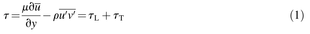
whereμandρare the dynamic viscosity and density of fluid,respectively;u is the velocity component in the main flow direction;v is the velocity component in the y-direction;“'”denotes fluctuations;“-”denotes the time mean values;andτ,τL,andτTare the total,viscous,and turbulent shear stresses,respectively.The term-ρu′v′is defined as the turbulent shear stress along the y-direction normal to the wall.Fig.1(a)and(b)shows the distributions of viscous and turbulent shear stresses and velocity as functions of distance from the wall in an open channel,respectively.The viscous shear stress is dominant in the vicinity of the wall(the wall layer),the turbulent shear stress is dominant in the outer layer,and there is an overlap layer in the middle,where both viscous and turbulent shear stresses are significant(White,2011).
The methods of shear stress distribution estimation from velocity distribution can be applied to irregular cross-sections or rivers.These methods do not require complicated mathematical calculations and powerful computers.It is generally necessary to obtain the velocity data through simple direct measurements or empirical models,and the velocity data are used to estimate shear stress.This study developed a new model to calculate the shear stress distribution along the wetted perimeter using the velocity distribution at the cross-section.
According to Eq.(1),shear stress estimation encounters problems in calculating turbulent shear stress due to the fluctuations of measured velocity.Considering the near-zero turbulent shear stress at the boundary(Fig.1(a)),the local bed shear stress(τ)in a smooth open channel at any crosssectional location is equal to the viscous shear stress at the location of the corresponding bed(Fig.1),and is expressed as follows:
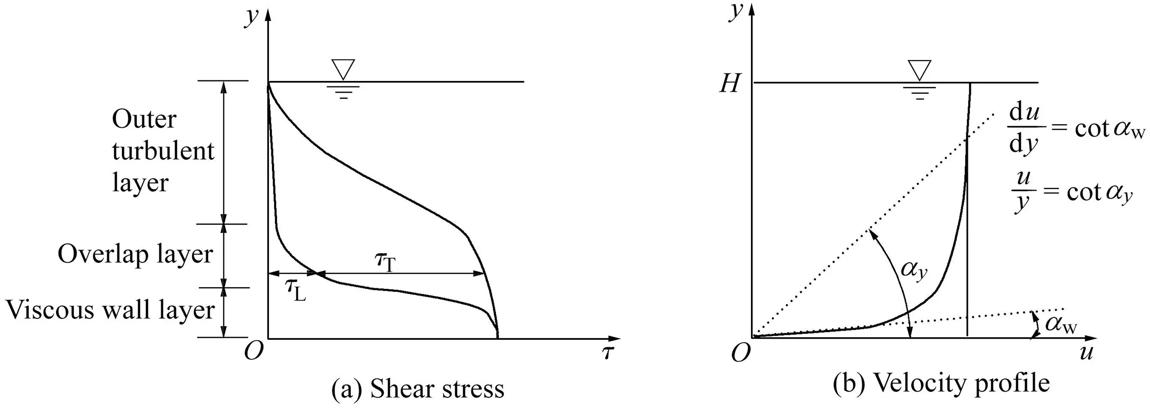
Fig.1.Typical shear stress and velocity distributions in developed turbulent flow near a wall.
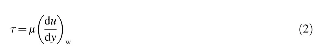
where the subscript w refers to the wall.When Eq.(2)is used to estimate the local boundary shear stress on the wetted perimeter,it requires measurement of the velocity gradient close to the wall((d u/d y)w).This is a formidable task because it is necessary to measure the velocity at some points very close to the boundary.Instead of using(d u/d y)w,the ratio of velocity to distance(u/y in Fig.1(b))was used to estimate the wall shear stress in this study.The proportion of these two velocity gradients(ξ)can be expressed as follows:

In the schematic turbulent velocity profile(Fig.1(b)),cotαwrefers to base slope.According to Eq.(3),ξcan be numerically estimated as the slope of the velocity gradient at the wall divided by the mean velocity gradient at a certain distance in the flow.By substituting(d u/d y)winto Eq.(2)with Eq.(3),the wall shear stress(τ)is obtained as follows:
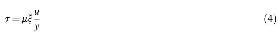
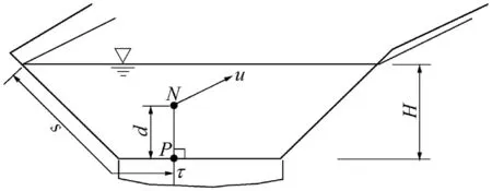
Fig.2.Specific parameters of proposed model at a cross-section.
In Eq.(4),y is the vertical distance from the bed.However,the aim of this study was to obtain the shear stress distribution along the wetted perimeter.Thus,the normal distance from the boundary(d)was used to replace y(Fig.2).According to Eq.(4),the velocity(u)at point N on the cross-section,its distance from the wall(d),and the dynamic fluid viscosity(μ)should be measured,and the only parameter required to calculate the shear stress at the corresponding point P on the boundary isξ.According to the experimental data,ξis not constant along a unique normal to wetted perimeter at a single point or on various normals at different points on the wetted perimeter.Hence,there are several pairs of u andτat a crosssection,and there is a uniqueξfor each pair.However,there are no theoretical or empirical methods to obtainξ.This study aimed at finding a general relationship between the velocity(u)at a point on the cross-section,the distance(d)from that point to the boundary,and shear stress(τ)at the corresponding point on the boundary in the form of Eq.(4).To obtain a unique general relationship for the model,the parameters of the crosssection,channel,and fluid specifications should be defined.
In an open channel,the mean bed shear stress along the wetted perimeter(τ0)is equal to the integrated values of the local shear stresses(τ)along the wetted perimeter,and it is obtained by the following equation:

where g is the gravitational acceleration,R is the hydraulic radius,and sfis the energy line slope.According to Eq.(5),shear stress on the wall(τ)depends on the fluid density(ρ),the area of the flow cross-section(A),the wetted perimeter(P),and the energy line slope(sf).Eq.(4)is basically reliable when only one wall is affected by the velocity distribution.However,for a cross-section with different restricted boundaries,the effect of other walls must be considered.Independent geometric cross-sectional parameters such as free water surface length(T),water depth(H),and distance along the wetted perimeter(s)(starting at the left bank on the free surface)are considered as well.The relationship could be expressed as follows:

In Eq.(6),all selected variables are independent except A,which is a function of T and H.Because this relationship varies from one section to another,A can be numerically independent in a general equation.For example,the defined function of A varies at different trapezoidal cross-sections that are dependent on the wall slope.Using the Buckingham Pi Theorem and substitutingξinto Eq.(4)with Eq.(6),ξcan be written as a function of seven dimensionless parameters:
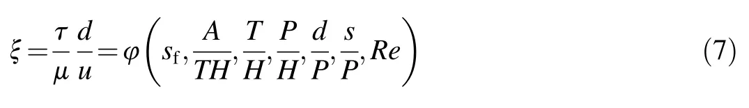
where Re refers to the Reynolds number.It is preferred thatξ be considered the products of their exponents.Given that there are different options for constructing dimensionless variables,some of them are selected through the trial-and-error method,andξis defined as follows:
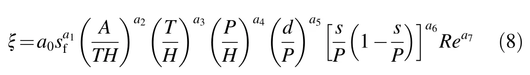
where a0,a1,a2,a3,a4,a5,a6,and a7are constants calculated with the regression method,and the exponents of two variables(s/P and 1-s/P)are selected identical,because the proposed formula must be valid in symmetric cross-sections.In the proposed model,y in Eq.(4)is substituted with d as described above.For eachτ,d,and u,the correspondingξcan be derived from the experimental data,and subsequently it is adopted to calibrate the proposed model as a function of the dimensionless channel parameters.
2.2.Experimental data
To evaluate the model,open channels with different crosssections that have been investigated by many researchers were considered in this study.As shown in Fig.3,these channels include rectangular and trapezoidal channels(Tominaga et al.,1989),trapezoidal and compound channels(Knight and Shiono,1990),and partially full circular channels(Knight and Sterling,2000).The model can be verified in the following channel conditions:(1) velocity distribution(perhaps in the form of isovel contours)is given at the crosssection,and(2)shear stress distribution is given along the wetted perimeter of the cross-section.The properties of these cross-sections are listed in Table 1.

Table 1 Properties of cross-sections.
At several points on each cross-section,velocity and shear stress are known.For each pair of points at the cross-section and on the boundary,the values of sf,d,H,T,P,s,A,and Re are known,andξwas calculated by the proposed model(Eq.(8)).Therefore,Eq.(8)is a parametric relationship with eight variables(a0,a1,a2,a3,a4,a5,a6,and a7).These variables were estimated by minimizing the statistical index,mean absolute percentage error(MAPE).

Fig.3.Rectangular,trapezoidal,compound,and partially full circular cross-sections for model calibration.
The minimization of MAPE for 60%of the recorded data in all cross-sections(or the mean value of MAPE for them)was selected as the objective function,and the remaining 40%of the data were used to validate the obtained relationship.The solution of this function can be written as follows:
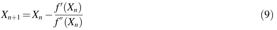
where Xnand Xn+1are the variables in the n th and(n+1)th steps,respectively,with m variables(m=8 in this study),and the functions f′(Xn)and f′′(Xn)are the gradient and Hessian of f(Xn),respectively.
3.Results and discussion
To estimate the eight variables(a0,a1,a2,a3,a4,a5,a6,and a7)in Eq.(8),it is necessary to consider the effects of initial values.After some trials,the best values of variables were selected for the first modeling step,considering the minimum MAPE value.The initial values of a0and a2were assumed to be 20 and 1,respectively,and the others were assumed to be zero.Fig.4 shows the variation of each variable normalized by its maximum absolute value as a function of the iteration number and the variation of MAPE.It shows that all variables reached a constant value after some variations,and MAPE decreased from 1.0 to 0.069 after more than 200 iterations.Therefore,according to Eq.(8),the calibrated relationship to calculateξis the following:

where the terms sf,A/(TH),T/H,P/H,and Re were calculated only once for the channel cross-section,and the two terms d/P and(s/P)(1-s/P)were calculated at each point on the boundary.Additionally,this equation can calculate an arbitrary point either on the bed or sidewalls without the need for any cross-sectional geometric treatments.Eq.(10)demonstrates that P/H was the most effective factor controllingξ.Additionally,ξwas inversely related to sf.In other words,if sfis magnified with other factors remaining constant,ξtends to decrease.
Although the mean MAPE value was approximately 0.069,it varied from section to section.Fig.5 shows theξ values calculated by the proposed model(Eq.(10))versus the measured values derived from Eq.(4)using the experimental data in all cross-sections.In a real situation,the measured and calculatedξvalues were not identical.A range of 10%error is shown in Fig.5.This figure shows that the proposed model provided good results in most cases,including thetrapezoidal cross-sections,the partially full circular crosssection,and one of the compound cross-sections,with MAPE values lower than 6%.This was mainly due to the nearly continuous wetted perimeter in these cross-sections without steep or right angles.In a partially full circular section with no angle or discontinuity in the wetted perimeter,the error was less than 10%at all points,and the effects of different points on the wetted perimeter were different at each point on the cross-section.The maximum MAPE value was 11.7%,and it corresponded to the rectangular crosssection(S2).For some points on this cross-section,the error was higher than 10%.The highest slope angle around the wetted perimeter was 90°.This produced a large discrepancy between the effects of two points near the wetted perimeter at any point on the cross-section.The good results shown in S1(another rectangular cross-section)were only relevant to the bed because the shear stress distribution data of the walls were not considered here.
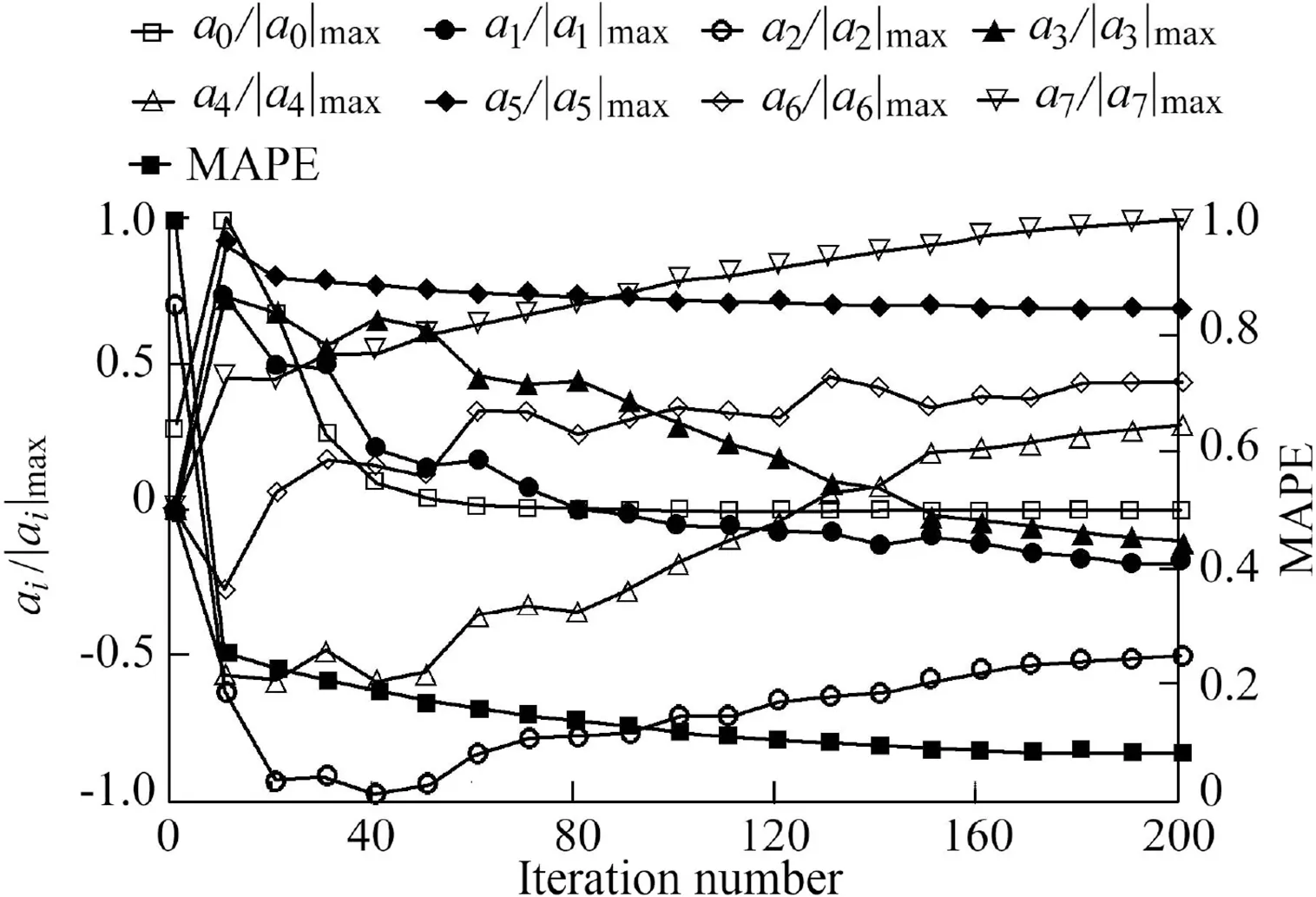
Fig.4.Variation of each variable normalized by its maximum absolute value and variation of MAPE.
To evaluate the feasibility of the proposed model in estimating the shear stress distribution,Fig.6 compared the measured shear stress distribution using experimental data against the calculated distribution derived from the proposed model,and both were normalized by the mean shear stress along the wetted perimeter(τave).As expected,the greatest similarity between the measured and calculated shear stress distributions appeared at the partially full circular cross-section,and the worst performance occurred at the rectangular cross-section(S2)and compound cross-section(030702_4).As indicated in Fig.6,for the rectangular cross-section(S2)located on the wall with s/P<0.1,the proposed model failed to estimate the shear stress by considering the velocity at each point.Similar results were found at the corner where s/P was approximately 0.16.However,at other regions of this cross-section,the model represented approximately accurate estimates of shear stress.Additionally,at the compound cross-section(030702_4),the modeling results were significantly different from the measured data in the case of s/P>0.4.At the trapezoidal cross-sections,the calculated results agreed with the observations.For the compound cross-section (030802_4),although the proposed model did not exactly capture the fluctuation of shear stress,the calculated shear stress showed relatively good agreement with the observations.
The intersection of the bed and wall in a corner simultaneously affected the velocity by the two boundaries,and this caused the poor results at the corners.Eq.(10)is a fundamental relationship of the proposed model,andξis a continuous function of s.Thus,the proposed model cannot estimate the effect of discontinuity of a wetted perimeter at the corners.The extreme discontinuity of the wetted perimeter at the corner of rectangular cross-sections(with an angle between the bed and wall of 90°)is an important factor for the high MAPE values.The lowest MAPE values were found at the partially full circular cross-section with no discontinuity in the wetted perimeter.
Given that shear stress at any point on the boundary can be estimated from the velocity at different points on the crosssection,Table 2 lists the error indices for the calculated mean shear stress values on the wetted perimeter against the measured values.
Table 2 shows that the lowest values of error indices were found at the compound(030802_4),trapezoidal(IB1501_1),and partially full circular cross-sections,and good results of the correlation coefficient were also found at these crosssections.As mentioned earlier,good values of indices for the rectangular cross-section(S1)were due to ignorance of the sidewall data.

Table 2 Error indices between measured and mean values of shear stress along wetted perimeter.
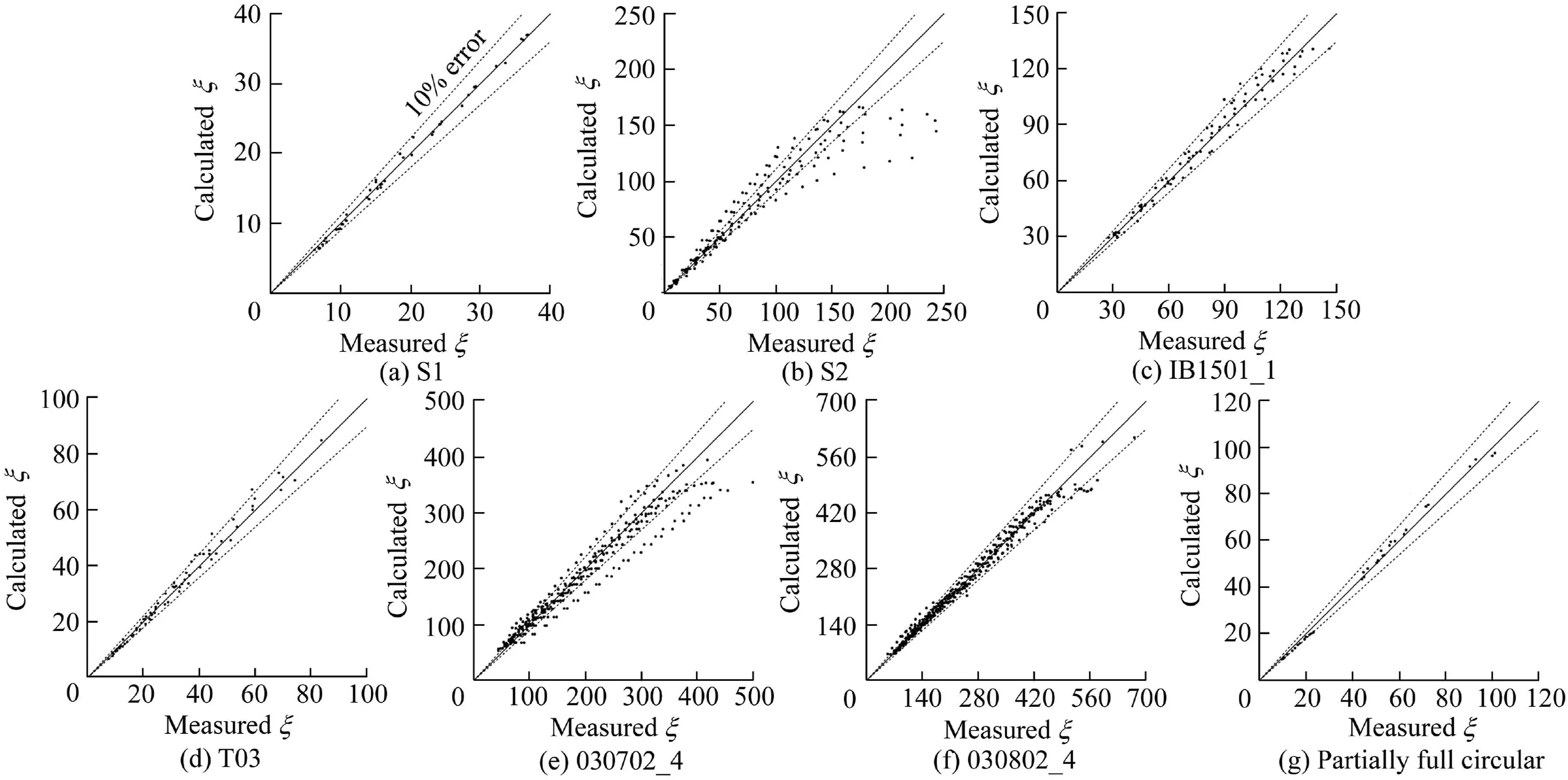
Fig.5.Calculatedξvalues versus measuredξvalues at seven cross-sections.
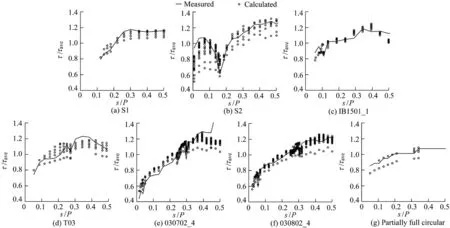
Fig.6.Calculated normalized shear stress distribution derived from proposed model versus measured distribution at seven cross-sections.
Finally,the 2D approaches were selected for comparison with the proposed model.Zarrati et al.(2008)derived semianalytical equations for shear stress distribution based on a simple streamwise vorticity equation including turbulent shear stress and secondary Reynolds stress.The analytical model of Shiono and Knight(1991)includes the effects of bed-generated turbulence,lateral shear turbulence,and secondary flows.This method and the analytical model of Zarrati et al.(2008)were applied to cross-section T03 and were compared with the experimental data of Tominaga et al.(1989).Given that this cross-section was also considered in this study,the distribution of boundary shear stress derived from the proposed and aforementioned models and the experimental data are shown in Fig.7.As indicated in Fig.7,although the results of the proposed model were close to the experimental data,the shear stress values for s/P<0.15 were overestimated in comparison with both analytical models.For s/P>0.2 on the wall,the predicted shear stress was located between those of two analytical models.Although the proposed model underestimated the shear stress for s/P>0.4 in comparison with the analytical models,it obtained relatively better results on the bed.The calculated MAPE between the proposed model and the experimental data was approximately 6%,and it was slightly higher than that of the model from Shiono and Knight(1991),which was approximately 5%.The estimated MAPE for Zarrati et al.(2008)was close to 10%,which was higher than that of the proposed model.
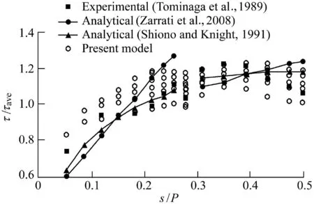
Fig.7.Boundary shear stress distribution presented by proposed model,experimental data,and two analytical models in cross-section T03.
4.Conclusions
In this study,a practical model was developed to estimate the boundary shear stress distribution.The proposed model does not require any complicated calculations.The dimensionless factor(ξ)was defined as a function of dimensionless variables of fluid and channel properties,and the proposed model estimated local boundary shear stresses along the wetted perimeter only using the viscous shear stress relationship.In this model,the shear stress distribution is related not only toξbut also to the velocity distribution at the crosssection.The multivariate Newton method was used to find the constant parameters of the relationship,and the minimum of the mean MAPE value between the model and the experimental data was selected as the objective function.After more than 200 iterations,the optimized variables reached constant values.The main conclusions are as follows:
The error between the calculated and measuredξvalues was less than 10%in most cases.The mean MAPE value was 6.9%,but MAPE varied across different sections.The largest MAPE with a value of 11.67%appeared at the rectangular cross-section with the highest amount of discontinuity in the wetted perimeter and with an angle between bed and walls of 90°.The lowest MAPE values of 4.3%were found in the cases of trapezoidal and compound cross-sections with no steep angles along the wetted perimeters.An MAPE value of 4.69%was obtained for the partial full circular pipe flow with no discontinuity along the wetted perimeter.In the partially full circular section,ξcan be accurately estimated by the model with MAPE values less than 10%at any point.The shear stress distribution along the wetted perimeter was calculated by the proposed model for all sections and compared with the measured distribution derived from the experimental data.Although there was a slight difference,especially at the walls and corners of rectangular and trapezoidal cross-sections,there was a relatively strong agreement between the model and the experimental data.Comparison between the proposed model and the 2D analytical methods of Zarrati et al.(2008)and Shiono and Knight(1991)for cross-section T03 demonstrated the feasibility of the proposed model.
These findings indicate that the proposed model helps the operators calculate turbulent shear stress without measurements of velocity fluctuations.Due to the viscous shear stress relationship,it is necessary to calculate the velocity gradient by measuring the velocity at several points near the boundary.However,when this model is adopted,a point at a considerable distance from the wetted perimeter can only be replaced by measurement of the flow velocity.
Declaration of competing interest
The authors declare no conflicts of interest.
 Water Science and Engineering2021年2期
- Water Science and Engineering的其它文章
- Flood disaster monitoring based on Sentinel-1 data:A case study of Sihu Basin and Huaibei Plain,China
- Influence of cascade reservoirs on spatiotemporal variations of hydrogeochemistry in Jinsha River
- Preparation and characterization of Fe2O3/Bi2WO6 composite and photocatalytic degradation mechanism of microcystin-LR
- Photodegradation of reactive blue 19 dye using magnetic nanophotocatalyst α-Fe2O3/WO3:A comparison study ofα-Fe2O3/WO3 and WO3/NaOH
- Enhancement of removal efficiency of heavy metal ions by polyaniline deposition on electrospun polyacrylonitrile membranes
- Assessment of physicochemical properties of water and their seasonal variation in an urban river in Bangladesh