
A STRONG SOLUTION OF NAVIER-STOKES EQUATIONS WITH A ROTATION EFFECT FOR ISENTROPIC COMPRESSIBLE FLUIDS?
2021-10-28 05:44TuoweiCHEN陳拓煒YongqianZHANG張永前
Tuowei CHEN(陳拓煒)Yongqian ZHANG(張永前)
School of Mathematical Sciences,Fudan University,Shanghai 200433,China
Email:16110180003@fudan.edu.cn;yongqianz@fudan.edu.cn
Abstract We study the initial boundary value problem for the three-dimensional isentropic compressible Navier-Stokes equations in the exterior domain outside a rotating obstacle,with initial density having a compact support.By the coordinate system attached to the obstacle and an appropriate transformation of unknown functions,we obtain the three-dimensional isentropic compressible Navier-Stokes equations with a rotation effect in a fixed exterior domain.We first construct a sequence of unique local strong solutions for the related approximation problems restricted in a sequence of bounded domains,and derive some uniform bounds of higher order norms,which are independent of the size of the bounded domains.Then we prove the local existence of unique strong solution of the problem in the exterior domain,provided that the initial data satisfy a natural compatibility condition.
Key words compressible Navier-Stokes equations;rotating obstacle;exterior domain;vacuum;strong solutions
1 Introduction
We consider 3-dimensional isentropic viscous gas flow past an obstacle that is a rotating rigid body with prescribed angular velocity.The gas occupies the time-dependent domain ?(t).Here,?(t)is de fined as

where

and ? is an exterior domain in R3with a smooth boundary.More precisely,we assume that R3? is compact,and R3?(t)can be regarded as an obstacle rotating around the x3-axis with a fixed angular velocity ω=(0,0,1).The fluid in our model is governed by the isentropic compressible Navier-Stokes equations in the time dependent exterior domain ?(t):
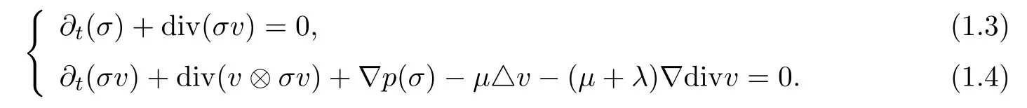
Here,t>0 is the time variable,and y=(y1,y2,y3)∈?(t)is the space variable.σ(t,y)and v(t,y)=(v1(t,y),v2(t,y),v3(t,y))denote the density and the velocity,respectively;p(σ)=Aσγ(A>0,γ>1)is the pressure;λ andμare the constant viscosity coefficients satisfying

The boundary conditions are

and

The initial condition is

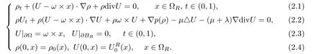
The above problem in a moving domain could be reduced to the one in the fixed domain?,as in[8,10,11,13].That is,we introduce the new unknown functions

where x=O(t)Ty.
Then,(1.3)–(1.8)could be reduced to the following:

There are many works on an incompressible flow surrounding a rotating body.For the autonomous case(in which ω∈R3{0}is a constant vector),Hishida[11,12] first constructed a local mild solution within the framework of L2,and later on,Geissert,Heck and Hieber[8]extended this result to the Lp-case.Hishida and Shibata[14]also showed the global existence for small data.For the non-autonomous case,the result of Hansel and Rhandi[10]may be regarded as a desired generalization of[8],and recently,Hishida[13]got some results for the global existence with small data.To the best of our knowledge,however,there is little in the mathematical literature about our subject for compressible flows with a rotation effect;see[6,17]for examples.In[17],Kraˇcmar,Neˇcasov′a and Novotn′y considered the motion of compressible viscous fluids around a rotating rigid obstacle when the density at in finity is positive,and proved the global existence of a weak solution.The regularities and uniqueness of such a weak solution remain open.In[6],Farwig and Pokorn′y considered a linearized model for compressible flow past a rotating obstacle in R3with positive density at in finity,and they proved the existence of solutions in Lq-spaces.
For the problem of a 3-D compressible Navier-Stokes system without a rotation effect,Matsumura and Nishida showed in[18,19]that the global classical solutions exist provided that the initial data are small in some sense and away from a vacuum.In the presence of an initial vacuum,in general,one would not expect general results for the global well-posedness of classical solutions due to Xin’s blowup result in[24],where it is shown that if the initial density has compact support,then any smooth solution to the Cauchy problem of the full compressible Navier-Stokes system without heat conduction blows up in finite time for any space dimension(see[2,26]for the cases with a boundary).For the isentropic case allowing for an initial vacuum,Choe and Kim[4] first showed the local existence of unique strong solutions by imposing,initially,a compatibility condition.We also recommend Cho-Choe-Kim[3]and the references quoted there in for readers to consult.In[3,4],to deal with the problem in an exterior domain and with an initial vacuum,Choe,Kim and Cho considered the related problem in bounded domains with the initial density having a positive lower bound,and by introducing a natural compatibility condition,they used the energy method to derive an a priori estimate for higher order regularity,which is independent of the lower bound of the initial density.They also showed that the uniform bound of their a priori estimate is independent of the size of the domain,so that they could use the domain expansion technique to obtain the desired result for the exterior domain.Recently,when the initial vacuum is allowed,a Beale-Kato-Majda blow-up criterion for the 3-D compressible Navier-Stokes equations was obtained in[20](see[5]for further results).For the global existence of classical solutions to the Cauchy problem of 3-D compressible Navier-Stokes equations with an initial vacuum,we refer the reader to[15,16,25]and the references therein for recent developments.
In this paper,we study the initial-boundary value problem(1.3)–(1.8)with the initial density having compact support,and we will show the local existence of unique strong solutions provided that the initial data satisfy a natural compatibility condition.Before stating our main result,we give a list of notations used in our paper.
For any domain M?R3,we denote

A detailed study of homogeneous Sobolev spaces can be found in[7].Without loss of generality,in our paper,we assume that R3??B1.
We now state our main result as follows:
Theorem 1.1Suppose that(ρ0,U0)satis fies

and
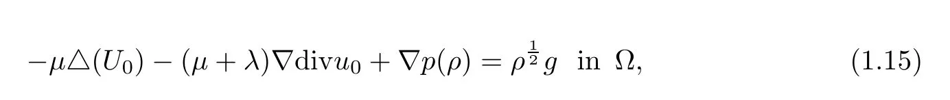
where R0is a positive constant and g∈L2(?)is a given function.Then there exists a small time T?>0 and a unique strong solution(ρ,U)to the initial boundary problem(1.10)–(1.13)such that

We have the following corollary concerned with the support of the density.
Corollary 1.2Let(ρ,U)be the solution given in Theorem 1.1.Then,ρ(t)has a compact support for t∈(0,T?)and satis fies

where C is a positive constant.
We remark that an essential difficulty to treating the exterior domain problem(1.10)–(1.13)lies in the growth at in finity of the coefficient in the term ρ(ω×x)·?U in(1.11),which comes from the rotation effect.This term creates difficulties for using classical energy methods as in[3,4]to derive uniform a priori estimates independent of the size of domain.In order to overcome such difficulties,we consider a sequence of bounded domains ?Rwith R→∞,and study the related linearized approximation problem restricted in ?Rwith the initial density having some special positive lower bound.Then,by using an energy method,we will derive some uniform bounds of higher order norms which are independent of R.Finally,we apply the domain expansion technique as in[3]to solve the original problem in the exterior domain.
The rest of this paper is organized as follows:in Section 2,we consider the linearized approximation problems restricted in a sequence of bounded domains ?Rand derive some uniform bounds of higher order norms which are independent of R.In Section 3,we apply the domain expansion technique to obtain the main results.
2 Existence Result for a Sequence of Domains ?R
In this section,we consider a sequence of domains ?Rwith R→∞and study the problem restricted in ?R.More precisely,we will show the local existence of a unique strong solution to the following initial boundary value problem with the initial density having compact support,and derive some uniform bounds of higher-order norms which are independent of size of ?R:
Here,for simpli fication,we consider t∈(0,1)as in[3,4].The initial data are assumed to satisfy the following assumptions:

Here C0is some positive constant independent of R.In addition,we assume that(ρ0,)satis fies the compatibility condition

for some g∈L2.
The main result in this section is stated as follows:
Theorem 2.1Let R>R0.Suppose that(2.5),(2.6)and(2.7)hold.Then there exist a small time T?∈(0,1)and a unique strong solution(ρ,U)to the initial boundary value problem(2.1)–(2.4)such that

Moreover,there exists a positive constant?C independent of R such that

Moreover,ρ(t)has a compact support for t∈(0,T?)and satis fies

2.1 Reduction of the problem
Inspired by[8,10,11,13],we fix a cut-offfunction ξ∈with support suppξ?such that 0≤ξ≤1 and ξ=1 near??,and put

Let

Then,the problem(2.1)–(2.4)is reduced to the following:

and that

both of which can be obtained directly by(2.6)and(2.7).
2.2 Linearized approximation problems
We consider the linearized approximation problems in two steps,as follows:
Step(1):De fine u0=0.
Step(2):Assuming that uk?1was de fined for k≥1,let(ρk,uk)be the unique solution to the following initial boundary value problem:

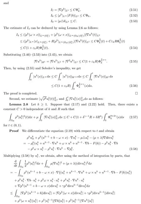
2.3 Uniform bounds
In this subsection,we will derive some uniform bounds independent of k and R on the approximation solutions(ρk,uk),and then prove the convergence of{(ρk,uk)}k≥1to a strong solution to problem(2.11)–(2.14).Throughout the remaining part of this section,we denote by C a generic positive constant depending only on R0,b,μ,λ,γ,A,C0,?,g,|ρ0|H1∩W1,6and,but independent of k and R.
Let k≥1 be an integer.For t∈(0,1),we de fine an auxiliary function Φk(t)by

We will estimate each term of Φk(t)in terms of some integrals of Φk(t),and then apply arguments of Gronwall-type to prove that Φk(t)is locally bounded.
We begin with some elementary observations on the Lq-norms(1≤q≤∞)of ρk.
Lemma 2.3For 2≤q≤∞and t∈(0,1),it holds that

and

Furthermore,the following inequality holds:

ProofSobolev’s inequality yields|ρk(t)|L∞≤CΦk(t).Then,from pk=A(ρk)γ,we also have.Hence,by taking interpolation,we obtain(2.24)and(2.25).

Thus,we can obtain(2.26)by similar arguments.
The proof is completed.
Lemma 2.4For 1≤q≤2 and t∈(0,1),it holds that

ProofBy virtue of the equation(2.18),we deduce the conservation of mass as

and it follows from(2.29)that

By taking interpolation again,we obtain(2.28).
The proof is completed.
Next,we state some regularity estimates for the so-called Lam′e system:


for some positive constant C=C(q,μ,λ,?)independent of R.
ProofSee Section 5 in[3];we also refer readers to the elliptic theory of Agmon,Douglis and Nirenberg in[1].
We now establish some estimates on the L∞-norm of ρkas follows:
Lemma 2.6Let ρkbe the unique solution of the equation(2.18)and let

Then the following estimate holds:


where C is a positive constant independent of k and R.
Proof(2.35)follows from the de finition of Φk(t)directly.To prove(2.34),note that for(t,x)∈(0,1)×?Rfixed,ρk(t,x)can be expressed by


In the next calculation,we will estimate all of the terms on the right hand side of(2.59).Among these terms,J4,J8,J10and J11,···,J13can be estimated by applying Lemmas 2.3 and 2.7 and by using Sobolev’s inequality and Hlder’s inequality as follows:

The terms J1,J3,J5,···,J7,J9,J18,···,J19and J22,···,J23can be estimated by applying Lemma 2.3 and Lemma 2.7 and by using Sobolev’s inequality,H¨older’s inequality and Young’s inequality as follows:
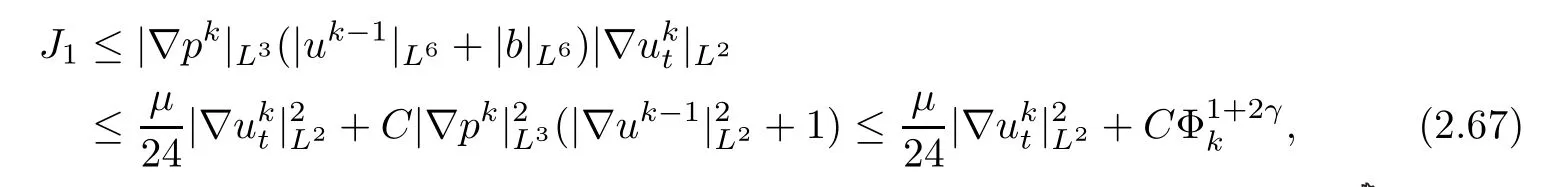

Finally,the terms J2,J14?J17and J20?J21can be estimated by applying Lemma 2.3,Lemma 2.7 and Lemma 2.6,and by using Sobolev’s inequality,H¨older’s inequality and Young’s inequality as follows:


In conclusion,(2.103)follows from(2.106)–(2.124).
The proof is completed.
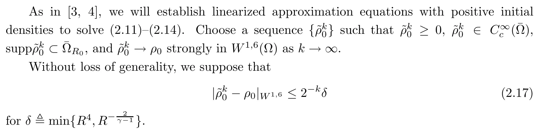
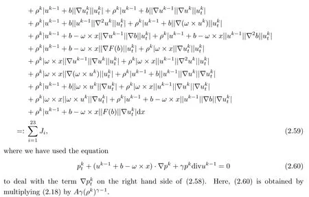
Lemma 2.10Let k≥1.Suppose that(2.17)and(2.22)hold.Then,there exists a constant C>0 independent of k and R such that

ProofSobolev’s inequality yields that

Thus,due to(2.42),it suffices to estimate|?2uk|L6.
Applying Lemma 2.5 to the elliptic system(2.44),we have

Here Q1,···,Q10can be estimated by applying Lemma 2.3 and Lemmas 2.7–2.9,and by using Sobolev’s inequality and Hlder’s inequality as follows:


Substituting(2.129)–(2.138)into(2.128),we obtain,after integrating the resulting inequality over(0,t),that
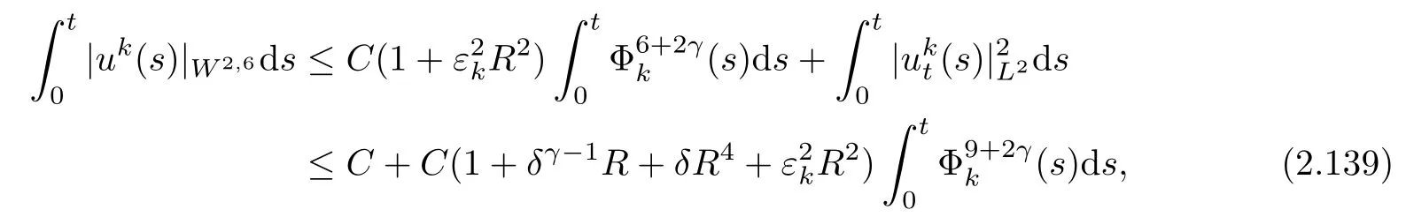
where we have used Lemma 2.8.
Therefore,Sobolev’s inequality,together with(2.139),gives

The proof is completed.
Finally,we estimate|ρk(t)|H1∩W1,6as follows:
Lemma 2.11Let k≥1.Suppose that(2.17)and(2.22)hold.Then,there exists a constant C>0 independent of k and R such that

for t∈(0,1).
ProofWe differentiate the equation(2.18)with respect to xjand obtain


Summing over the above for all j,we get

which implies that


Hence,with the help of Lemma 2.7,Lemma 2.10 and(2.92),Gronwall’s inequality provides(2.141)from(2.146).
The proof is completed.
Now,we are in a position to derive the uniform bounds on Φk(t).Combining Lemmas 2.7–2.11 together,we obtain

Applying Gronwall’s inequality to(2.147),we find a small time T0>0 and a constant C>0,both of which depend only on R0,b,μ,λ,γ,C0,A,?,g,but which are independent of k and R such that

where we have used(2.42)and(2.125).Therefore,we have the following:
Proposition 2.12Let k≥1.Suppose that(2.17)and(2.22)hold.Then,there exists a constant C>0 independent of k and R such that the strong solution(ρk,uk)to(2.18)–(2.21)satis fies the above estimate(2.148).
2.4 Convergence
We are ready to show that the full sequence(ρk,uk)of approximation solutions converges to a solution to the problem(2.11)–(2.14)in a strong sense as follows:
Proposition 2.13Suppose that(2.17)and(2.22)hold.Then,there exist T?∈(0,1)independent of R and a weak solution(ρ,u)to the problem(2.11)–(2.14)on(0,T?)×?Rsuch that

ProofLet k≥1,and let

Then,it follows from(2.18)–(2.19)that


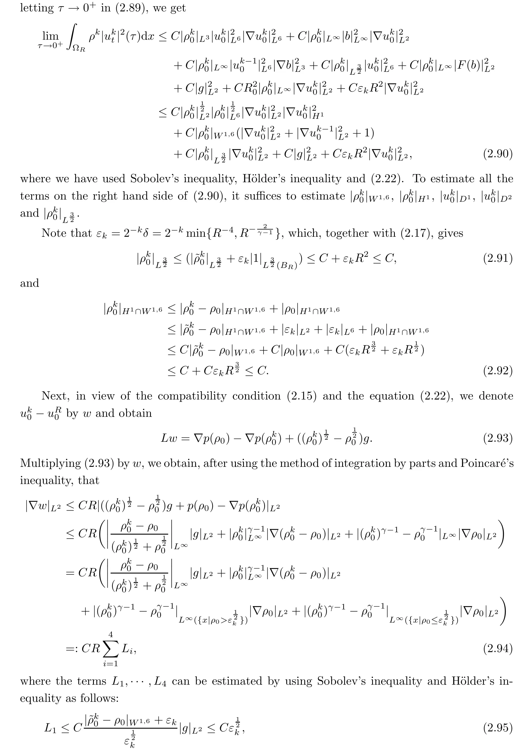
To estimate all the terms on the right hand side of(2.154),we first focus on the termBy Lemma 2.6 and(2.148),we have

Thus,by using Sobolev’s inequality and Young’s inequality,and by(2.148)and(2.155),we deduce from(2.154)that


which,together with Gronwall’s inequality,gives

where C is a generic positive constant independent of N and R.
Hence,there exists(ρ,u)such that

and it is easy to check that(ρ,u)is a weak solution to the problem(2.11)–(2.14),as in[3].
The proof is completed.
2.5 Proof of Theorem 2.1
Now we are in a position to prove Theorem 2.1.
Proof of Theorem 2.1Let(ρ,u)be the weak solution to(2.11)–(2.14)given in Proposition 2.13 and let U(t,x)=u(t,x)+b(x).Then,(ρ,U)is a weak solution to problem(2.1)–(2.4).Moreover,by virtue of the lower semi-continuity of norms,it follows from(2.148)that(ρ,U)satis fies the estimate

Carrying out the same arguments as in the proof of Lemma 2.6,we use(2.166)to obtain that ρ(t)has a compact support for t∈(0,T?)and satis fies

In addition,the time-continuity of(ρ,U)can be proved by the standard arguments as in[3].As for the uniqueness of strong solutions to(2.11)–(2.14),these can be obtained by using a similar method as in the proof of Proposition 2.13.
The proof is completed.
3 Existence Result for the Exterior Domain
We are in a position to prove our main theorem.


Finally,noticing(3.5),by an analogous argument as to that of Section 2,it is easy to check that(ρ,U)is indeed a unique local strong solution to(1.10)–(1.13).
The proof is completed.
To conclude,we prove Corollary 1.2 as follows:
Proof of Corollary 1.2Since U∈L∞(0,T?;W1,6(?)),with the help of Sobolev’s inequality,we could obtain(1.16)by using the same approach as to that used in the proof of Lemma 2.6.
The proof is completed.
 Acta Mathematica Scientia(English Series)2021年5期
- Acta Mathematica Scientia(English Series)的其它文章
- RIGIDITY RESULTS FOR SELF-SHRINKING SURFACES IN R4?
- GLOBAL STRONG SOLUTION AND EXPONENTIAL DECAY OF 3D NONHOMOGENEOUS ASYMMETRIC FLUID EQUATIONS WITH VACUUM?
- CONTINUOUS TIME MIXED STATE BRANCHING PROCESSES AND STOCHASTIC EQUATIONS?
- SOME OSCILLATION CRITERIA FOR A CLASS OF HIGHER ORDER NONLINEAR DYNAMIC EQUATIONS WITH A DELAY ARGUMENT ON TIME SCALES?
- COARSE ISOMETRIES BETWEEN FINITE DIMENSIONAL BANACH SPACES?
- ZERO KINEMATIC VISCOSITY-MAGNETIC DIFFUSION LIMIT OF THE INCOMPRESSIBLE VISCOUS MAGNETOHYDRODYNAMIC EQUATIONS WITH NAVIER BOUNDARY CONDITIONS?