Variational quantum simulation of thermal statistical states on a superconducting quantum processer

Xue-Yi Guo(郭學儀), Shang-Shu Li(李尚書),2, Xiao Xiao(效驍), Zhong-Cheng Xiang(相忠誠),Zi-Yong Ge(葛自勇),2, He-Kang Li(李賀康),2, Peng-Tao Song(宋鵬濤),2, Yi Peng(彭益),2,Zhan Wang(王戰),2, Kai Xu(許凱),4, Pan Zhang(張潘), Lei Wang(王磊),8,?,Dong-Ning Zheng(鄭東寧),2,4,8,§, and Heng Fan(范桁),2,4,9,?

1Beijing National Laboratory for Condensed Matter Physics,Institute of Physics,Chinese Academy of Sciences,Beijing 100190,China

2School of Physical Sciences,University of Chinese Academy of Sciences,Beijing 100190,China

3The Chinese University of Hong Kong,Shatin,New Territories,Hong Kong,China

4CAS Center for Excellence in Topological Quantum Computation,University of Chinese Academy of Sciences,Beijing 100190,China

5Institute of Theoretical Physics,Chinese Academy of Sciences,Beijing 100190,China

6School of Fundamental Physics and Mathematical Sciences,Hangzhou Institute for Advanced Study,University of Chinese Academy of Sciences,Hangzhou 310024,China

7International Centre for Theoretical Physics Asia-Pacific,Beijing/Hangzhou,China

8Songshan Lake Materials Laboratory,Dongguan 523808,China

9Beijing Academy of Quantum Information Sciences,Beijing 100193,China

Keywords: superconducting qubit, quantum simulation, variational quantum algorithm, quantum statistical mechanics,machine learning

1. Introduction

Hybrid variational quantum–classical algorithms(VQAs)[1]are recently proposed to solve quantum manybody problems by taking advantages of both classical algorithms and quantum resources. The main idea is to arrange the classically high-cost computational part to the quantum co-processors and use well developed classical optimizers to find solution. Such approaches are feasible on near-term noisy intermediate-scale quantum(NISQ) devices for robustness in the presence of noise and decoherence.[2–4]VQAs have been extensively demonstrated for solving ground states of quantum systems known as variational quantum eigenstate solver(VQE)[5–12]and have important applications such as solving combinatorial optimization problems[13,14]and simulating general time evolution problems.[15,16]Thermal states and highly excited states have attracted more interest for their importance in studying novel non-equilibrium phenomena[17–21]of quantum many-body systems. It is of great significance and also challenging to directly prepare these states on a quantum computer. Some progress has been made in preparing Gibbs states[22–33]and excited states[34–38]using quantum computers. However, there are few experimental implementations especially for preparing arbitrary specified highly excited states,and the system size is generally limited due to the scalability problem. For example,approaches accessing thermal Gibbs ensemble by variationally preparing thermal field double states[26,28]require an approximate measurement of entropy, which takes extra experimental resources. Quantum imaginary time evolution (QITE)[30]suffers from an inefficiency with deep circuits at low temperatures or large system sizes. It is also challenging to extract physical observables from an exponential large mixed state in a scalable way.

Here we present our implementation of a general variational algorithm for quantum statistical mechanics problems[32,33,39]on a 5-qubit superconductor quantum processor and show its potential to solve the above issues. The algorithm takes the combination of classical generative models and quantum circuits as variational ansatz and performs classical optimization,which can be regarded as a finite-temperature generalization of VQE. Compared with other algorithms for thermal state preparations,[28–31]the classical representation of the mixture probabilities reduces the burden of the quantum processor, has an advantage of efficiently estimating the entropy with small or even no statistical error, and benefits from the methods and models rapidly developed in machine learning. Consequently,the combined approach is particularly feasible for NISQ implementations.

We experimentally prepare Gibbs states and all eigenstates for HeisenbergXXchain andXXZchain with high fidelities using an improved gradient-based optimizer. Our approach can be scaled up to larger systems benefiting from a small number of samples in each training step and shallow quantum circuits. We evaluate the performance of our approach using state tomography, where the target Gibbs state can be constructed with fidelity reaching 92.6%. Moreover,we illustrate that the classical probability can help us prepare arbitrarily specified eigenstates, of which the highest-fidelity reaches 98%. We also demonstrate that the approach has a self-verification property[11]and can reduce statistical error in the calculation of fundamental thermal variables.

2. Methods

2.1. The hybrid quantum–classical variational approach

In general,the thermal density matrix of a target quantum system can be represented as a classical mixture of pure states.The pure states can be prepared by applying a parameterized unitary quantum circuit ?Uθon a set of input state{|x〉}, and the classical mixture can be realized by using a probabilistic generative model. This gives an hybrid ansatz[32,33]for the thermal density matrix,

where the set{|x〉}denotes the computational basis,pφ(x)is the parameterized probability distribution model satisfying∑x pφ(x)=1 andUθis the variational quantum circuit. The variational parametersθ,φare determined by minimizing the distance between ?ρand target density matrix ?σ= e-β?HT/Z,where ?HTis the Hamiltonian of the target quantum system,βdenotes the inverse temperature,andZ=Tr(e-β?HT)is the partition function. The Gibbs–Delbr¨uck–Moli′eve variational principle of quantum statistical mechanics[40]suggests to take the variational free energy?=(1/β)Tr(?ρln ?ρ)+Tr(?ρ?HT)as the loss function,which is lower bounded by the true free energy with equality holds only when ?ρ= ?σ.

Using the variational ansatz in Eq. (1), the loss function is written as

where we have defined|ψθ(x)〉= ?U(θ)|x〉. The loss function can be separated into the energy term and the entropy term. The energy evaluation Ex～pφ(x)[〈ψθ(x)| ?HT|ψθ(x)〉]can be performed efficiently with the help of a quantum processor for preparing|ψθ(x)〉. While for the entropy term Ex～pφ(x)[lnpφ(x)]which is difficult to estimate using quantum computer,it now can be evaluated purely classically based on a proper probabilistic model on binary variablex. There are two ways to obtain the expectation in Eq.(2)which corresponds to the thermal average. When the number of qubitsNis small,pφ(x)can be exactly characterized by storing probabilities for totally 2Ncomputational basis vectors, and the thermal average is done using all the basis and corresponding probabilities. We term this as the full-space method. Apparently, the computational cost of this approach is exponential inN. Alternatively,a scalable way is to represent the probability distribution by a parameterized generative model and evaluate the thermal observables with sample mean,which we term as the sample method.

Here we use the sampling method combined with a classical gradient-based optimizer to optimize the hybrid variational model in a mini-batch gradient descent manner. At each step of the optimization, a set of bitstrings{x}are sampled frompφ(x)generating initial states|x〉as inputs to the quantum circuitUθ. After applying unitary transformations,the outputs of the quantum circuit work as final states|ψθ(x)〉, using which we measure energyEθ(x)=〈ψθ(x)| ?HT|ψθ(x)〉.Together with the entropy estimated solely usingpφ(x),we compute the loss function and its gradients, then employ an efficient classical optimizer to update the parameters. The overall classical–quantum optimization process is sketched in Fig.1(a).

For classical optimization, we adopt a gradient-based method that is particularly feasible for training the combination of probability model and general quantum ansatz. Due to the large fluctuations of the loss function estimated using a small number of samples, the gradient-free optimizers such as the Nelder–Mead simplex method, particle swarm algorithm, Bayesian optimization,[41]and the dividing rectangles optimizer[11]are not suitable for our task. In this work, we consider the gradient-based optimization scheme, with gradients computed as

In general,one cannot compute directly the gradients with respect to the model parameters, so we need to use the score function gradient estimator

whereR(x) = lnpφ(x)/β+〈ψθ(x)| ?HT|ψθ(x)〉,bdenotes a base line parameter to reduce the variance,[33,42–45]and we adopt a common choice thatb= Ex～φR(x). Details about the evaluation of gradients (3) and (4) can be found in Appendix D.

For the classical distribution, in consideration that the number of qubits is small, we use a product of Bernoulli distribution for each qubit

whereφi ∈[0,1] is the probability thatxibeing 1. Each Bernoulli distribution is further parameterized using the sigmoid function with a single variableφi(αi)=1/(1+e-αi).The gradients forφare then derived“semi-classically”,where the evaluation of ?φlnpφ(x) is done on a classical computer whereR(x) andbcontain the energy values measured using the quantum circuit. In the experiments,we observed that the product distribution already has enough expressive power for the system with five qubits. It is straightforward to replace the product distribution with a more powerful probabilistic model,e.g., the autoregressive model as adopted in Ref. [33] which has much more parameters and a better representation power than the product distribution,by taking advantage of the deep learning techniques.

Fig.1. Thermal variational quantum simulation on a superconducting quantum processor. (a) Feedback loop of the hybrid quantum–classical variational algorithm in our experiment between the classical process unit (CPU) and the quantum process unit (QPU). A classical probability distribution pφ(x) is maintained using classical computational resources,producing bitstring samples{x}which work as the input product states|x〉for QPU.The QPU performs several layers of unitary quantum circuits U(θ)with the input product states and produces the final states by which the energy Eθ(x)is estimated.The energy is forwarded to the CPU for evaluating the loss function and its gradients for the parameters of pφ and Uθ. Then a classical optimizer is employed to update the parameters upon which new bitstring samples are generated for the next loop until the loss function converges. (b) False-color image of our quantum device. There are five frequency-tunable transmon qubits laid at the middle of the chip, each of them has a readout resonator, an XY control line, and a Z control line. All the five readout resonators are coupled to a readout transmission line. See Appendix Table A1 for the basic characteristics of qubits. (c)Pulse sequence for the quantum circuit ansatz for a certain input state(|x〉=|10101〉).The evolution of the global entanglement layer(with the XY couplings)persists 9 ns. The amplitude tunable square pulses of 25 ns are used to realize the parameterized Rz(θ). After d-layer evolutions(d=5 in our experiment),the-X/2,Y/2,or I gates are applied for each qubit for the energy measurement.

2.2. Model and device

We focus on the spin-1/2XXandXXZHeisenberg chains in a magnetic field, which are prototype models studied extensively in condensed matter physics. The Hamiltonian can be written as

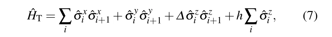
where ?σx,y,zare Pauli matrices. The model has a globalU(1)symmetry corresponding to the conservation of the total spin on thezdirection. In the limit withΔ= 0, the model reduces to theXXmodel, which can be mapped to the freefermion model by Jordan–Wigner transformation and thus exactly solvable.

Our experiments build upon a quantum processor with five frequency-tunable transmon qubits[46–48](see Appendix A for experimental details) arranged in a line with nearest-neighbor couplings, whose false-color image is presented in Fig.1(b). The qubit chain can be modeled as a onedimensional spin-1/2 model withXXinteractions, of which the Hamiltonian is expressed as

3. Results

3.1. Experimental optimization for XX model

Here, we train the variational circuit by applying the quantum–classical algorithm for 500 iterations as illustrated in Fig.1. The experimental optimization results forXXmodel atβ=0.5 are presented in Fig.2. In the experiments,we take 2 samples in each learning step which is much smaller than the dimension of the Hilbert space 25. We show that such a small sample size is already enough for the optimization process,see Fig.2(a). The performance of the learning from sampling can be checked by re-evaluating the loss function using the full space method. The corresponding full space re-evaluated optimization curve is also shown in Fig. 2(a). We can see that the loss function given in both experiments and noisy numerical simulations decreases from a large initial value to a value that is about 5% higher than the exact free energy at the end of learning. This error can be explained by our experimental error model (see Appendix B) since the experimental results are in good agreement with our noisy numerical simulation results. The final parameters ofUθandpφare determined using theθ*,φ*values corresponding to the minimal loss in the full-space re-evaluation curve. Practically,one should use the loss evaluated by the sample method since it avoids exponential cost. However, when the optimization cannot find the optimal value as in our noisy experimental case, the variance of loss is generally rather large and the sample method is hard to determine the optimized parameters.Nevertheless,it can be used when the optimization terminates successfully due to the self-verification feature discussed below.

Figures 2(b)–2(c) present the probability distributionpφ*(x) and experimentally measured energyEθ*(x) for each participate states|x〉. They are in coincidence well with the exact distributionPGibbs(n)= e-βEn/Zand the eigen energiesEn. For comparison, we also perform an ideal noiseless simulation with exact quantum gates. The results are shown in Appendix Fig. E2, where the probability distribution and the eigen energies match the exact values very closely, indicating that our quantum circuit can fully diagonalize the target Hamiltonian in the noiseless case.

The small sample number used in both experiment and ideal simulation implies an exponential reduction of computational complexity. We confirm this by a numerical study and show that the total time cost grows polynomial in qubit number (see Appendix D). Another property that can be clearly shown in the experiments is the self-verifying feature from the sample variance. It is shown both experimentally (Fig. 2(a))and theoretically (Appendix Fig. E2) that the variance of the sample curve decreases as the loss function during the optimization(see the inset of Fig.2(a)). This is because that when the learning is exact,the variance should be zero. Thus empirically we can use the sampling variance of the loss function as the self-verifying indicator(see Appendix C2 for more discussion). Moreover,this indicator can be accessed directly in the experiment hence avoiding extra complex measurement that is needed in the ground state VQE algorithm.[11]

3.2. Preparation of Gibbs states and excited states

We experimentally construct the Gibbs states by state tomography of each component state and present the results in Fig. 3(a). The measured density matrix is transformed to the eigenbasis{|n〉}of the target Hamiltonian. We obtain a Gibbs state whose fidelity is 92.6% to the exact Gibbs state. Furthermore, since in our approach the probability of each state can be determined and the Hamiltonian is fully diagonalized by ?U(θ*). We can hence distinguish excited states(up to degenerations)using their probability values. More specifically,the exact eigenstate|n〉corresponding to|ψθ*(x)〉is identified using the bitstring withn-th largest probability inpφ*(x).This allows us to experimentally prepare both the ground state and any specified excited states of the target Hamiltonian,after running the optimization only once. In Fig. 3(b), the density matrix ?ρxof several experimentally prepared excited states in the eigenbasis{|n〉}together with the corresponding initial basisxare presented.The results involve states at both edges and the middle of the spectrum. We observe that each density matrix has the largest amplitude located at the correct entry in the density matrix, with high fidelity to the corresponding exact density matrices. The full fidelity matrix between the experimentally prepared eigenstates|ψθ*(x)〉and the exact eigenstates|n〉is illustrated in Appendix Fig.E3.

Fig.3. Density matrices of the Gibbs states and eigenstates obtained in the experiments for XX model. (a)The density matrix of the obtained Gibbs states ?ρ*(upper panel)compared with the exact Gibbs states(lower panel),the fidelity is 92.6%.(b)Density matrix ρx of experimentally prepared eigenstates|ψθ*(x)〉,where the corresponding exact eigenstate|n〉is identified by the nth probabilities pφ*(x)sorted in a decent order. In all the plots,only the amplitudes of the density matrix are shown,with diagonal elements and off-diagonal elements colored by red and blue,respectively.

3.3. Thermal observables estimation

In Fig. 4, we show the experimental estimation of internal energy and thermal entropy according toE=Ex～pφ(x)[〈ψθ(x)| ?HT|ψθ(x)〉] andS= Ex～pφ(x)[lnpφ] respectively by sampling method. These observables generally have larger statistical variance than the free energyFand cannot be estimated precisely with a small number of samples. The same situation is also encountered in other approaches,e.g.,in Ref.[31].Here we propose to resolve this issue by utilizing the thermodynamic relationE=F+(1/β)S, based on the selfverifying feature ofFand the classical estimation of entropyS.Self-verification of free energyFensures its small variance at the optimal point,while the entropyScan be accurately evaluated by classical methods(see Appendix C1). In this way,the variance of the energy estimation can be greatly reduced. It is extendable to any thermal quantities which can be expressed as a function of free energy and entropy. In Figs. 4(a)–4(c),we plot the thermal quantities obtained in experiments where the entropy is computed using an analytical method with no statistical error and the free energy is evaluated using 5 samples. The variance of energy is at the same level as those of free energy and entropy, which are much smaller than those obtained in existing methods. From Fig.4(d),the standard error for internal energy obtained by the sampling method with 200 samples is even larger than that obtained by our improved approach with five samples. Thus,our strategy is efficient for large-scale problems.

Figure 4 also shows that our approach can successfully prepare Gibbs states and obtain thermal quantities in a wide range of temperatures, particularly when compared with existing approaches. For example,the truncated entropy approach[29]is limited to low-temperature regions due to the series truncation of entropy. The long imaginary evolution time in QITE[30,31]for a low temperature (β ＞0.5) leads to fast-growing circuit depth and error accumulation. In contrast,our algorithm uses a quantum circuit with a fixed depth,hence is not influenced significantly by the temperature. It works all the way down toβ=3.0 as shown in Fig.4.

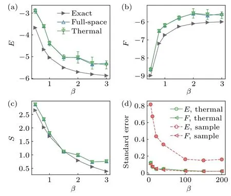
Fig.4. Thermal quantities obtained by experiment at different inverse temperatures. The internal energy (a) and free energy (b) derived by full-space(up triangle) and thermal relation approach (down triangle). In the latter method, the sample size is 5 and the error bars are obtained as the standard error by repeating the evaluation 20 times. (c)The entropy is evaluated using an analytical expression hence contains no statistical error. (d)Standard error of experimental derived internal energy and free energy as a function of sample number,using sample(dashed)and thermal(solid)approach.

3.4. Results for XXZ model

Finally, to further demonstrate the performance of our variational approach, we apply the same method to the spin-1/2XXZchain withh=0,which is an interaction model and has an additional Z2symmetry.We find that ourU(1)preserving quantum circuit also produces reliable results for theXXZchain with the model parameters we studied (see Appendix Fig. E1), indicating that our method is general for studying different quantum lattice models.

4. Conclusion

We have demonstrated the hybrid quantum–classical variation approach on a superconducting quantum processor for solving quantum statistical mechanics of the quantumXXandXXZchains. The method utilizes the generative probabilistic modeling in machine learning for maintaining the mixture distribution and estimating the variational entropy classically,combined with the quantum processor for performing unitary transformations and estimating the energy. The parameters of the generative model and quantum circuits are learned through a scalable mini-batch gradient-based method. Taking advantage of both classical and quantum resources,we have shown that the variational approach can prepare Gibbs states and arbitrary excited states for theXXandXXZmodels with high fidelity. It also has a self-verifiable feature using the variance of the loss function, and can estimate thermal quantities with a small statistical error.

Our approach is general and flexible for extensions. The quantum circuits can be readily updated to near-term quantum devices with a much larger size,and the classical distribution can be generalized to more representative neural network generative models straightforwardly.[33,45]On the application side, the proposed approach can be extended immediately to other condensed matter models such as the Fermion systems using the Jordan–Wigner transformation. Moreover, with the prepared Gibbs states, we can further investigate the finitetemperature dynamics on quantum simulators.[31]Last but not least,the preparation of eigenstates at certain energy densities also makes it possible to study many-body localization[19,20]and eigenstates thermalization hypothesis[17,18]with quantum computers.

Appendix A:Experimental details

A1. Experiment setup

Our quantum device is placed at 10 mK in a BlueFors dilution refrigerator. It is well screened from the higher temperature environment with its own aluminum alloy package box and a magnetic shield. Outside of which, we have another layer of aluminum alloy shield and magnetic shield at 10 mK.All these shields are tightly sealed and well thermally connected to the 10 mK plate. The control wires connected to the quantum device are deeply attenuated and filtered against noise from the room temperature environment and electronic setups. ForXYcontrol lines,[48]we have 3 dB attenuation at 40 K,20 dB attenuation at 3 K,6 dB attenuation at 800 mK,and 40 dB attenuation at 10 mK,plus a 7.5 GHz low pass filter.ForZcontrol lines,[48]we use a capacitance removed bias-tee at 10 mK to combine the DC bias and fastZsquare pulse.For the fastZcontrol lines,we have 3 dB attenuation at 40 K,20 dB attenuation at 3 K, 6 dB attenuation at 800 mK, and 10 dB attenuation at 10 mK, plus a 500 MHz low pass filter before connected to the bias-tee. We use continuous 0.86 mm CuNi coaxial cables as our DC bias lines, and apply an RC low-pass filter at room temperature, whereR=1 kΩ, and a 200 MHz low-pass RLC filter at 10 mK before connecting to the bias-tee. For the input line of readout pulses,we have 3 dB attenuation at 40 K,20 dB attenuation at 3 K,6 dB attenuation at 800 mK,and 40 dB attenuation plus a 7.5 GHz low-pass filter at 10 mK.For the output line of readout pulses,we have a Josephson parametric amplifier(JPA)at 10 mK,a HEMT amplifier at 3 K, and another microwave amplifier at room temperature. We isolate our quantum device from the JPA with a 7.5 GHz low-pass filter and an isolator. We have another isolator between the JPA and HEMT.

Room-temperature electronic instruments are used to generate stable direct current, microwave pulses, and current pulses to control and readout states of qubits. Here, we use Yokogawa GS220 as a DC voltage source to bias qubits to their idle frequencies, the output range is set to 1 V. Zurich Instrument HDAWGs are used to generate microwave pulses via IQMixers,and to generate current pulses as fastZcontrol pulses.

Table A1. Qubit characteristics. is the zero flux biased frequency of Qi. ωi is the idle frequency of Qi. is the readout resonator frequency of Qi. T1,i is the energy relaxation time of Qi at the idle frequency. is the dephasing time of Qi at the idle frequency. U/2π is the nonlinearity(f21- f10) of Qi measured at the zero flux bias. F1,i (F0,i) is the measured probability of|1〉(|0〉)when Qi is prepared in|1〉(|0〉). gi,j is the coupling strength between Qi and Qj.

Table A1. Qubit characteristics. is the zero flux biased frequency of Qi. ωi is the idle frequency of Qi. is the readout resonator frequency of Qi. T1,i is the energy relaxation time of Qi at the idle frequency. is the dephasing time of Qi at the idle frequency. U/2π is the nonlinearity(f21- f10) of Qi measured at the zero flux bias. F1,i (F0,i) is the measured probability of|1〉(|0〉)when Qi is prepared in|1〉(|0〉). gi,j is the coupling strength between Qi and Qj.

Q1 Q2 Q3 Q4 Q5 ω0i /2π (GHz) 5.531 4.968 5.433 4.999 5.502 ωi/2π (GHz) 5.435 4.932 5.378 4.975 5.471 U/2π (MHz) –242 –196 –239 –196 –242 T1,i (μs) 31 35 35 36 54 T*2,i (μs) 9.14 7.39 7.27 8.74 12.64 g1,2/2π (MHz) 14.60 g2,3/2π (MHz) 14.65 g3,4/2π (MHz) 14.17 g4,5/2π (MHz) 14.26 g1,3/2π (MHz) 1.142 g2,4/2π (MHz) 0.607 g3,5/2π (MHz) 1.207 ωri/2π (GHz) 6.612 6.654 6.687 6.7266 6.766 F0,i 0.98 0.97 0.97 0.97 0.99 F1,i 0.91 0.88 0.89 0.89 0.89

The basic characteristics of qubits are listed in Table A1.Compared to the previous experiment,[46]the idle frequencyωiof each qubit is closer to its sweet point. With this idle frequency setup, the dephasing timesat idle points of 5 qubits can reach 7 μs–12 μs. The average energy relaxation timeT1at idle points of five qubits is 38.2 μs. While the resonant coupling frequency in this experiment is 4.932 GHz. To tune all five qubits from their idle frequency to 4.932 GHz,the output range forZcontrol channels of our Zurich Instrument HD is set to 2 V instead of 800 mV from its direct mode. We found that this change brings little effect to the dephasing time of the qubits.

Generally, the variational optimization process is robust to coherent errors while still is affected by random interference and noise from the environment. With this experimental setup, we monitored the fluctuation of the idle frequency for days during the experiment and found that the fluctuation of all 5 qubits is in the range of [-0.1,0.1] MHz, as shown in Fig. A1. This fluctuation amplitude is close to the adjustable precision of our experiment setup.[46]

Fig. A1. Fluctuation of the qubit idle frequencies. We have monitored the idle frequency of all qubits and found that the fluctuations are in the range[-0.1,0.1] MHz, which is close to the adjusted precision of our room temperature electronic system.

A2. Preparation of computational basis states

In the experiments, the input states for the quantum circuits are chosen from the set of computational basis{|00000〉,...,|11111〉}, which are generated with combinations ofXigates.We use the optimization methods in Ref.[47]to reducing the phase error ofX,X/2, andY/2 gates used in our experiment. Preparing multi qubits in|1〉suffers from the unwanted cross-talk affection induced by multiXgates, and the residual coupling between qubits. These effects reduce the fidelity of the prepared states. The measured fidelity of all 25input states is presented in Fig.A2.

Fig. A2. Fidelity of the input states. The 25 computational basis states are prepared using a combination of X gates and the fidelity of the states is measured. Preparing multi qubits in|1〉suffers from the unwanted crosstalk affection induced from multi X gates and the residual coupling between qubits which reduce the fidelity of the prepared states.

A3. Constructing parameterized quantum circuit

The variational quantum circuit is constructed by layers of global entanglement gate and single-qubitRzrotation gates.To realize the entanglement gate,fast square pulses are applied to tune all qubits to the same frequency for～9 ns,corresponding to dimensionless timeτ=π/4.With the measured step response function of each fastZcontrol line,we can compensate and correct the distortion of the applied square pulses,meanwhile,eliminate the fluctuations after the square pulses.[46]

The programable single-qubit gates in the experiments are realized using theRzgates,by tuning the qubit frequency with amplitude tunable square pulses of duration 25 ns. TheRzgates are calibrated using the Ramsey-like experiments.We insert anRzgate between twoπ/2 pulses. For a given amplitude of theRzgate,the phase of the secondπ/2 pulse is verified to determine the rotation angle,which results in a function of the rotation angle and pulse amplitude,using which we can set the required rotation angle ofRz(θ) in our experiments.The cross-talk between theZcontrol lines is experimentally determined and compensated so that theRzgates for different qubits have no affection to each other.[46]

A4. Energy expectation determination

For the input states with more than one qubit in an excited state,the implementation of a global entanglement gate can induce the state leakage to|2〉,as described in the last section.To reduce the state-leakage error,we measure all qubits simultaneously under the qutrit computational basis.Thus,the dimension of the measured Hilbert space is 35,i.e.,from|00000〉to|22222〉. Then,we reduce and normalize the measured Hilbert space to 25under the qubit computational basis,by discarding the results of one or more qubits in|2〉. The influence of this leakage error for the algorithm is discussed in Appendix B.It should be pointed out that such state-leakage error induced in resonant interaction-based entanglement gates could be effectively reduced by using non-resonant interaction-based entanglement gate schemes, such as conditional-phase gates based on tunableZZ-interactions.[49]

Appendix B: The error model for the quantum device

Here we discuss the error model for the real-device numerical simulation. The Hamiltonian Eq.(8)used in the main text is an approximate version of the real quantum device Hamiltonian. There are two intrinsic reasons that make the simulations on the hardware deviate from the ideal simulation results. One reason is the extra small couplings between the next-nearest neighbor qubits(see Table A1). Since our entanglement layer is realized in an analog way,the numerical simulation results show that in the presence of next-nearest neighbor couplings the ansatz has a poorer expression of the target model. The problem can be resolved by using two-qubit gates to realize entanglements. The other reason is the state-leakage error from non-infinite anharmonicity of the transmon qubit,where our device should be modeled by the Bose–Hubbard model with a large on-site interaction. The state-leakage error not only increases the measurement error of the observables but also prevents us from accessing regions with a very high temperature. The issue comes from the requirements of unitarity of the quantum circuit ?Uθfor evaluating the entropy part in loss function classically. To extract the spin observable with a measured 35dimensional density matrix, we abandon the probabilities that one or more qubits are excited to the|2〉states, leading to an effective non-unitary circuit. The nonunitary effect causes inaccuracy in the classical computation of entropy and destroys the variational principle. At high temperatures, the effect is more serious since the entropy plays a more important role in the loss function. Thus we present the results withβ ≥0.5,where the optimizations can proceed effectively.

There are mainly several possible resources contributing to the statistical errors in the measurements of observables.The first one is the measurement error when using many single-shot measurement results to calculate observables. The second one is the experimental random noise that leads to parameters fluctuation such as the idle frequency drift(Fig.A1).The first error can be efficiently simulated while the latter is hard. But they both effectively generate random noise in observable evaluations. So in the simulations, we use smaller single-shot measurements to effectively simulate these two errors. Another error resource is the decoherence process. Our circuit is shallow, the total operation time for the quantum gate is much less than the decoherence timeT1andT2(see Table A1), so we neglect the decoherence effect in the realdevice simulations.

Appendix C:Details on the variational algorithm

C1. Thermal observable calculations

After learning,the thermal observables such as the internal energyEcan be computed as a function ofpφandUθ,using a large number of samples than those in the learning process. The self-verifying feature implies that when the obtained variational free energy is close to the exact values, the small variance of the samples allows us to accurately estimateFusing a small number of samples. Remarkably, since entropy estimation only relies on the classical distribution using a generative model,observables such as the entropy which are hard to compute on quantum computers can be estimated efficiently classically usingpφ(x). In particular, benefit from the product distribution ansatz ofpφ(x)=∏i pφi(xi), we are able to evaluate the entropy with no statistical error using an analytical expression

If the classical distribution is implemented using a more representative model such as the autoregressive neural networks,[33]one can still use a polynomial algorithm to generate a large number of samples for estimating the entropy, resulting in a much smaller statistical error than that of energy which requires access to a quantum resource. For example,one could parameterize the joint distribution as a product of conditional probabilities

Here we need to pre-determine an order for the variablesx.This is actually the chain rule of probabilities, also known as the autoregressive model.[43]As a simple example,let us consider a simple example with 4 binary variables

pφ(x1,x2,x3,x4)=p(x4|x1,x2,x3)p(x1,x2,x3)

=p(x4|x1,x2,x3)p(x3|x1,x2)p(x1,x2)

=p(x4|x1,x2,x3)p(x3|x1,x2)p(x2|x1)p(x1). (C3)

At the first glance, some of the conditional probabilities are still difficult to express due to an exponential number of parameters to the number of variables in it. In practice,one can adopt an efficient model such as neural networks with a polynomial number of parameters to the number of variables for parameterizing the conditional probability. There are two essential properties of this representation,the ability to compute normalized probabilitypφ(x) for any configurationx, and a fast sampling algorithm. The first property is obvious because each conditional probability is normalized as

which means thatpφ(x) is naturally normalized. The second property is known as ancestral sampling,[50]which samples variables one by one given that we have stored every normalized conditional probability. Again taking the example with 4 variables,we can first toss a coin to fix a configuration forx1according top(x1), then toss a coin to fix a configuration forx2according top(x2|x1), and configurations forx3andx4in turn. Moreover, a large number of unbiased samples can be drawn in this way parallelly.

Equipped with the properties,one can easily make an accurate estimate of entropy using

where in the last equation we have usedmsamples to approximately estimate the expectation value.Thus,given the thermal relationF=E-(1/β)S,we can computeEmore accurately with a much smaller statistical error than estimating it directly using samples.

C2. Variance and the self-verifiable feature

The loss function used in the optimization is the variational free energy

which is evaluated as a mean value over the variational distribution.Its variance usually offers additional information about the confidence of optimizations. This is based on the fact that the variance is zero when the learning is exact. To illustrate this,suppose the optimization is perfect such that?equals the exact free energyFandpφ(x) characterizes exactly the level statisticP(x),with

with energy computed as

Then we can see that

which is independent ofx, indicating that the variance of〈ψθ(x)| ?H|ψθ(x)〉is zero. However, when we encountered a zero-variance during learning which produces the zero gradients of the loss funciton with respect to the model parameters,it does not indicate that the learning is exact. To see this,suppose

withCdenoting a constant,one has

This means that when the zero-variance condition is reached,the learned distribution is a Boltzmann distribution. However notice that eβCdoes not necessarily be eβF, resulting in a Boltzmann distribution that deviates from the true distribution.This is usually due to the model collapse effect that the variational ansatz can only explore part of the configuration space.

Nevertheless, in practice, the amount of variance can be used to justify and verify the quality of learning. Empirically,a small variance usually indicates a small variability of model prediction, yielding a small gap between the variational free energy and the exact free energy,e.g.,in theβ-VQE[33]algorithm and its classical counter part.[45]

Appendix D:Optimization method and scalability

D1. Gradient descent method

Here we describe the detail of the gradient descent method. To estimate the gradients of the energywith respect to parameters of the quantum circuitθ(which are the parameters of the single-qubit rotation gates in our set up),we could employ the parameter shift rule(PSR),[51]which only requests the loss function values at a forward and backward shift ofπ/2 for each parameter. However, it is inefficient for a quantum circuit containing a large number of parameterized gates and has limitations when the variational gates do not satisfy the PSR condition. Another popular method to estimate the gradients is the simultaneous perturbation stochastic approximation (SPSA) algorithm.[52]It approximates the gradients of the loss function for all parameters simultaneously by taking only two values of the loss function in a perturbation way,hence has a constant time complexity regardless of the number of gates or shape of quantum circuits. However, in the experiments, we observed that the computational cost of pure SPSA methods depends on the number of iteration stepsniterto achieve the desired accuracy,which follows a power-law scaling and has a high chance of trapping into local minima of the loss function.

In this work, we use a hybrid gradient descent optimization scheme by combining the SPSA with the adaptive moment estimation (Adam)[53]optimizer, denoted by SPSAAdam. In the algorithm, the exact gradients in the Adam optimizer are replaced by the mean of several SPSA gradient estimations.[52]The hybrid optimizer combines together the advantages from the compatibility of the SPSA gradients and the fast convergence in the noisy environment from the Adam optimizer. We will show that the number of SPSA trailsnSPSAfor obtaining the average gradients has a polynomial scaling to the number of qubitsN.

D2. Numerical results on scalability

Now we present an analysis of the computational complexity of the variational algorithm in numerical simulations with qubit numberNranging from 4 to 10. There are several classical optimization schemes depending on which gradients it uses, e.g., the sampling method or the SPSA gradients. The optimizers have different hyperparameters giving different performance and resource costs. We determine the hyperparameters and corresponding resource cost for a given precision starting from the algorithm containing a minimum number of hyperparameters. First,by using the full-space approach and the precise gradients derived by parameter shift,denoted as the full-space PSR-Adam optimizer,we determine the scaling of circuit depthnlayerwith respect to qubit numberN. Next, by selecting the value ofnlayeron the contour line of a certain precision, we employ the sampling version of PSR-Adam to determine the scaling of cost with different sample sizesnbatch. Finally, withnlayerandnbatchdetermined in the above steps, the scaling behavior of sampling SPSAAdam scheme is studied,where an additional hyperparameternSPSA,denoting the average number of SPSA gradient evaluation,is considered. The final cost of the optimization scheme shows a polynomial growth,which means that our approach is scalable for large systems. Although the results are obtained under a target model of theXXchain,the experimental and numerical results for theXXZmodel(see Fig.E1)confirm that the scaling is the property of the optimization algorithm rather than the target model,hence we expect that the scaling is universal for other complex models. Here we present details of the scaling analysis on theXXmodel where bothhandβare set to be 0.5.To save computational resources in both time and space,we did not consider noises in the numerical simulation.

D3. Full-space PSR-Adam

The most important hyper-parameter is the number of layernlayerwhich is critical to the expressibility and entangling capability of the quantum circuits. Using the full-space PSR-Adam optimizer, we study the relationship between the obtained loss function as a function of the layer numbernlayerranging from 3 to 10 in the simulations. The number of iterationniteris set to 150, which is beyond the iteration steps required for convergence in the case of the full-space scheme.We plot the relative errorsε=for different layer numbernlayerand qubit numberNin Fig.D1(a). We chose a precision threshold that the relative error is within 0.5%. Under the criterion, the scaling of the circuit depthnlayeris approximately linear indicated by the dashed line in Fig.D1(a).In the experiments,in order to balance the expressibility with the noise and decoherence error,we setnlayer=5 in the quantum circuits.

D4. Sampling PSR-Adam

The computational cost for each specific optimizer mainly comes from the evaluation of the gradient of the loss function with respect to the parameterθ’s. For the PSR-Adam scheme, the cost is proportional to the number of parametersnpara. With the sampling scheme,the gradient forθtakes the following form:

Fig. D1. Determining the optimal layer number nlayer and the mini-batch size nbatch for the PSR-Adam optimizer. (a) Relative error ε with N and nlayer ranging from 3 to 10 after 150 iterations of the full-space PSR-Adam optimization steps. Each point is averaged over 10 trials. The dashed line indicates the minimum value of nlayer that has an averaged error below 0.5%.The minimum nlayer has an approximately linear scaling in the qubit number.The optimal layer number is determined as nlayer =5 for N =5 in the experiments, as the circuit representation ability is powerful enough while the circuit is not so deep in order to reduce the decoherence effects. (b)Computational cost of the sampling PSR-Adam optimization as a function of N with nbatch =2,6,10 with ε less that 1.0%. The results are averaged over converging runs(iteration steps niter ＜1000)from 20 trials. In the inset of(b),the lnN–lncost plot is close to a straight line. This indicates that the growth of computational cost follows a polynomial scaling instead of an exponential one,and nbatch=2 is the most economic choice for the mini-batch size.

A small constantnbatchwith respect to the increasing system size gives an exponential reduction to the complexity of the variational algorithm for each iteration since the full-space scheme would require 2Nterms in the sum.However,the sampling scheme would require a larger number of iterations. We consider the total cost for PSR-Adam optimizer with sampling scheme as

withnlayerset according to the contour in Fig. D1(a). Given fixednlayerandnbatch,we record the number of iterationsniterrequired to reach the precisionε ＜1.0%. Taking into account the randomness that comes from the random initial parametersθand the stochastic optimization process, we have used 20 trials for the sameNandnbatchand calculate the statistical average of the converging runs, i.e.,niter＜1000. The maximal iteration steps 1000 is considered to be large enough since only 1 trial is labeled as‘divergent’among 420 trials in total.We present the results for differentnbatchin Fig. D1(b). For the precision threshold and qubit number we considered here,it seems thatnbatchcan be any integer larger than one. This is because the increasing computation complexity in thenbatchsector can be converted to the computation complexity manifested in the largernitervalue, while maintaining the value ofnbatch. Thus,it appears to be a trade off betweennbatchand the number of iterationsniter. A largernbatch, in general, renders a smallerniterfor the lost function to reach a fixed precision.However, we found that the complexity spared by a smallernitercould not balance out the extra cost from largernbatch.As a result,it turned out to be the most efficient choice to setnbatch=2 in both numerical and experiment implementation.

In the inset of Fig.D1(b),we show the scaling of the total cost with respect toNfornbatch=2. We fit the data both with power-law cost ∝NbA,which is plotted in the lnN–lncost coordinate. We observe that the slope in the lnN–lncost scatter plot follows a straight line with slopebA=2.51,indicating a polynomial scaling.

D5. Sampling SPSA-Adam

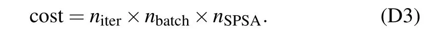
Here we consider the case of the SPSA-Adam optimizer,where the evaluations of the gradient with respect to all parameters are replaced by simultaneous shifts in all parameters averaged overnSPSAtimes. Thus the cost is proportional tonSPSAand can be estimated as

We set the mini-batch sizenbatchto 2,as determined in the last subsection, and investigate the scaling of computational cost viaN. The SPSA average numbernSPSAis selected from{1,3,5,7,9,11,13}and each set of hyperparameters is trialed 20 times. We record the averaged number of iterationsniterrequired for each value ofNto reach the precisionε ＜3.0%.The maximumniteris set to 1500.Any trial withniterexceeded the maximalniteris considered divergent,and the corresponding parameternSPSAis considered to be too small for the correspondingN.

Similar to the relation betweennbatchandniter, there appears to be a trade off wherenitertends to decrease asnSPSAincreases. The parameternSPSA,however,does have a different scaling behavior fromnbatch, where we found thatnbatch=2 is always the most efficient option. Starting fromN=6 withnSPSA=1,N=9 withnSPSA=3,andN=10 withnSPSA=5,there are cases where the value ofnitersurpassed the maximum iteration limitniter=1500. As a consequence,those data were not calculated and missing in Fig. D2, as we consider those value ofnSPSAare below the minimum threshold for the corresponding qubit number.

The scaling of computational cost is shown in Fig. D2,where the dashed line represents the minimum cost required for eachNwithε ＜3.0%. The scaling of the minimum cost is also plotted in a lnN–lncost in the inset. It again illustrates a power-law behavior cost ∝NbSwithbS=3.26.

As shown in Figs. D1(b) and D2, the SPSA-Adam optimizer has a scaling of higher-order compared with the PSRADAM optimizer even with lower precision.The result agrees with theoretical analysis that the zero’s order or gradient approximating methods have higher-order scaling in terms of both increasing qubit number and precision, compared with optimizations using analytic gradient measurements.[54]We only investigated the scaling result of SPSA-Adam optimization forε ＜3.0% but not for higher precision due to limited computational resources.

Fig. D2. Scaling of the computational cost for the SPSA-Adam optimizer with an increasing qubit number N. Computational cost with increasing N for nSPSA =1,3,5,7,9,11,13 with ε less than 3.0%. Given a fixed precision, there is a threshold for nSPSA for each N and therefore the curves corresponding to different nSPSA terminate at certain values of N. The dashed lines indicate the minimal cost simulated for each N. The results are averaged over converging runs(iteration steps niter ＜1500)from 20 trials. In the inset,the lnN–lncost plot of the minimum cost is close to a straight line and the slope, i.e., bS =3.26 corresponds to the exponent of the growth if the growth was assumed to be polynomial, i.e., cost ∝NbS. This indicates that the growth of the computational cost follows a polynomial scaling instead of an exponential one.

However,the SPSA-Adam optimizer is shown to be more efficient than the PSR-Adam optimizer in this experiment as the former only takes a few (in this experimentsnSPSA=10) averages compared withnpara=25 parameters for PSRAdams optimizer. Moreover, the SPSA-Adam optimizer will always hold the advantage when certain symmetry, e.g., parity or translation symmetry, is implemented in the circuit, as the same parameter applies to different quantum gates. The parameter shift method would not benefit much from the symmetry implementation whereas the SPSA method for calculating the gradient would reduce a considerable amount of cost in such cases.On top of that,parameter shift rules have their limitations especially when dealing with gates that do not square to a constant time the identity, while the SPSA method will not be limited by the choice of quantum circuits ansatz, thus has an advantage over the PSR-Adam optimizer.

Appendix E: Additional experimental and numerical results

In this section,we present the experimental optimization results forXXZmodels(Fig.E1),ideal numerical simulation results forXXandXXZmodels (Fig. E2), and experimental obtained fidelity matrix forXXandXXZmodels(Fig.E3).

Fig.E1. Experimental optimization results for quantum XXZ model with h=0,Δ =0.3,and β =0.5. (a)Optimization trajectory(light blue)and full-space re-evaluation results(blue)of the loss function with the sampling scheme and the SPSA-Adam optimizer. The shaded area denotes the standard error of 50 full-space re-evaluations with the mean(teal)at the center. The black dashed line is the exact value of free energy. The inset shows a self-verify indicator by tracking the sample variance of the loss function. Optimized probability distribution pφ*(x)(b)of the Gibbs ensemble and eigenenergy Eθ*(x)(c)of the target Hamiltonian with parameters θ*,φ* corresponding to the iterative step marked by the star in(a). The energy expectations are sorted by probabilities.The density plot of eigen energies in (c) is obtained from 50 numerical simulations. (d), (e) Density matrix of the Gibbs states and eigenstates obtained experimentally for the quantum XXZ model. (d) The density matrix of the optimized Gibbs states ?ρ* (upper panel) compared with the exact Gibbs states(lower panel). (e)Density matrix ρx of prepared specified eigenstates|ψθ*(x)〉,where the corresponding exact eigenstate|n〉is identified by nth probabilities pφ*(x)sorted in a descending order. In all plots,only the amplitudes of the density matrix are shown. The diagonal elements and the off-diagonal elements are colored by red and blue,respectively.

Fig.E2. Ideal numerical optimization results. (a)–(c)Results for the quantum XX model with h=0.5,β =0.5. (a)Optimization trajectory(shallow blue)and full-space re-evaluation results(blue)of the loss function with the sampling scheme and the SPSA-Adam optimizer.The shaded area denotes the standard error of 50 ideal numerical trials of the full-space re-evaluated optimizations,with the mean(teal)at the center. The black dashed line is the exact value of the free energy. The inset shows a self-verify indicator by tracking the sample variance of the loss function. Optimized probability distribution pφ*(x)(b)of the Gibbs ensemble and the eigen energy Eθ*(x)(c)of the target Hamiltonian with parameters θ*,φ* corresponding to the iterative step marked by the star in(a). The energy expectations are sorted by probabilities and show a one-to-one correspondence with the exact value. The density plot of the eigen energies in(c)is obtained from 50 ideal trails. (d)–(f)Results for the quantum XXZ model with h=0,Δ =0.3,and β =0.5. Due to the limited expressive power of our variational ansatz for the XXZ model,some eigen energies identified by probabilities deviate from the exact values,which are also shown in Fig.E3.

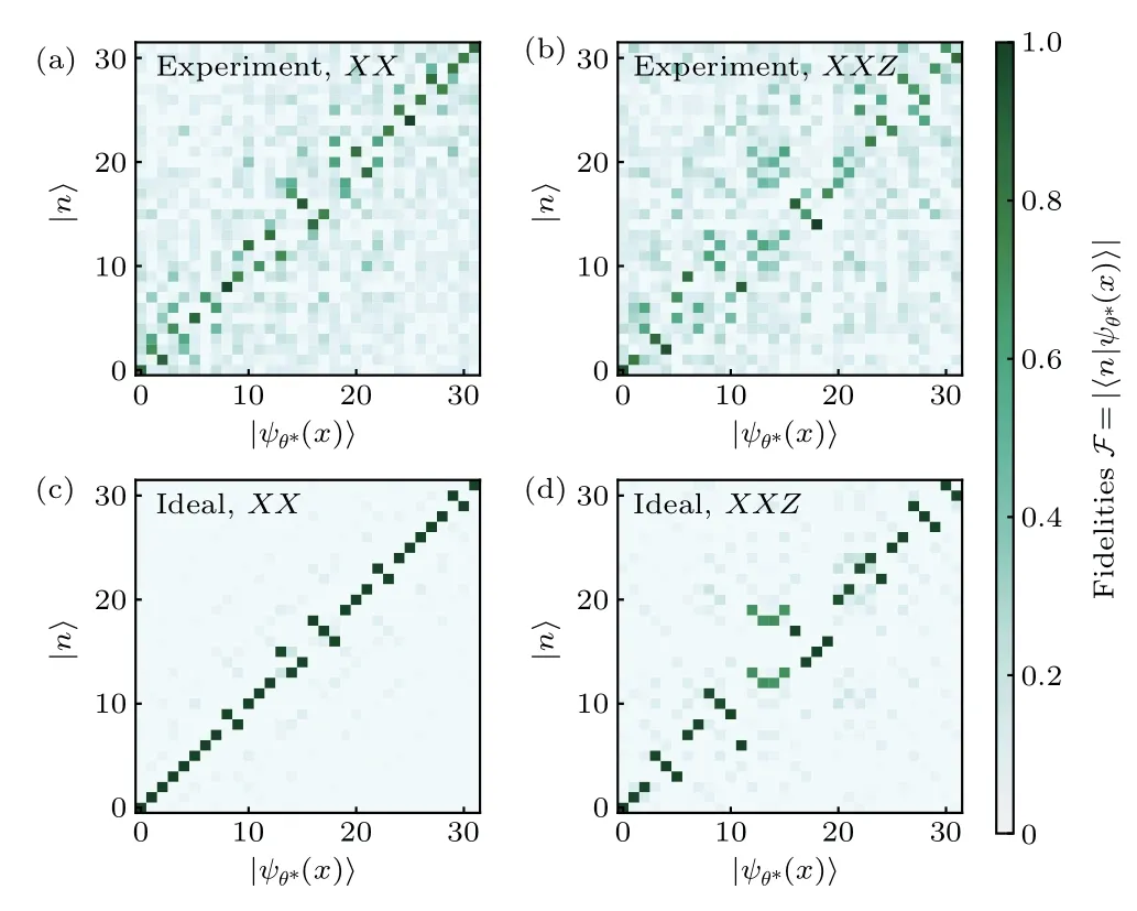
Fig.E3. The fidelity matrix between the optimized eigenstates|ψθ*(x)〉and the exact eigenstates |n〉. (a), (b) The fidelity matrix for the XX and XXZ model obtained in experiments. The matrix elements are concentrated near the diagonal entries, indicating that the eigenstates of the target Hamiltonian are prepared accurately in the experiments. (c), (d)The fidelity matrix from the ideal simulations for the quantum XX and XXZ model,respectively.In the XX case,most matrix elements are exactly diagonal-located while the off-diagonal elements represent the degeneracy of the target energy spectrum.For the XXZ model,the elements that deviated from the diagonal entries are given by both the degeneracies and the in-exact correspondence between the probability-identified eigen energy and the exact eigen energy.

Acknowledgments

We thank Zhengan Wang, Ruizhen Huang and Tao Xiang for useful discussions. Project supported by the State Key Development Program for Basic Research of China(Grant No. 2017YFA0304300), the National Natural Science Foundation of China (Grant Nos. 11934018, 11747601, and 11975294), Strategic Priority Research Program of Chinese Academy of Sciences (Grant No. XDB28000000), Scientific Instrument Developing Project of Chinese Academy of Sciences (Grant No. YJKYYQ20200041), Beijing Natural Science Foundation (Grant No. Z200009), the Key-Area Research and Development Program of Guangdong Province,China(Grant No.2020B0303030001),and Chinese Academy of Sciences(Grant No.QYZDB-SSW-SYS032).