
Investigation of replacing tracer flooding analysis by capacitance resistance model to estimate interwell connectivity
2023-08-30 03:25AdiletAliyevDvoodZivrPeymnPourfshry
Petroleum 2023年1期
Adilet Aliyev ,Dvood Zivr ,Peymn Pourfshry ,*
a School of Mining and Geosciences,Nazarbayev University,Astana,Kazakhstan
b PanTerra Geoconsultants B.V,Leiderdorp,Netherlands
ABSTRACT Interwell connectivity is an essential parameter for managing waterflooding operations in a field.Analysis of the tracer injection operation is a well-known approach to studying injected fluids distribution in a reservoir and toward producer wells.Developed in the early 2000s,capacitance-resistance model (CRM) is an analytical approach for waterflooding modeling and optimization.Production/injection data are used as input to model the mass balance and estimate parameters such as the interwell connectivity.In this work,we investigated the accuracy of applying the capacitance-resistance model to mimic a tracer test.Such an approach helps assess the connection between the wells and decide on further field development steps cheaper and quicker.Connectivity values estimated by tracer tests and CRM were analyzed and compared for synthetic and real fields.CRM was capable of modeling waterflooding and estimating production in both fields with acceptable accuracy.Parameters such as well spacing and fluid loss during the injection were considered to improve the accuracy of the CRM approach to calculate the interwell connectivity between injector/producer pairs.Our study showed that CRM could serve as a tool for a quick approximate estimation of interwell connectivity under certain assumptions and is recommended as a replacement for tracer flooding analysis,where the tracer test is not possible or is expensive.
1.Introduction
Interwell connectivity between injectors and producers is a crucial parameter to evaluate the performance of different oil recovery methods such as water flooding.Accurate knowledge of interwell connectivity parameters is essential for reservoir management and field development strategies.Assessing subsurface fluid channels,pathways,oil saturation and well-to-well connections helps characterize the reservoir better and reduce uncertainty in reservoir models,eventually leading to enhanced field operations.For example[1],showed for the net/gross ratio of higher than 30%,the stratigraphic connectivity is greater than 90% for channelized reservoirs,which highlights importance of such assessments.
Tracer technology is used for monitoring and surveillance purposes,and tracers are injected into a reservoir to study fluid flow parameters in the porous media,such as a well-to-well connection[2].The direct demonstration of communication in the connected pore space of a reservoir is an evident piece of information that may be obtained via tracers.Connections are determined by comparing the produced mass versus injected mass,analyzing the tracer breakthrough time,and investigating when most of the tracer has arrived.These parameters provide valuable information on the sweep efficiency and the fluid flow in reservoirs.Tracer data analysis gives a better picture of the reservoir flow and essential parameters such as injector/producer connectivity.This analysis provides valuable information on the sections of the reservoir swept,the velocity of the fluid in the porous media,and the effect of each injector on producers.Evaluation of tracer production in different producers helps us determine the presence of highly permeable channels and fractures,communication between different layers,and stream directions in the porous media.Knowledge of interwell connectivity is more critical in more complicated reservoirs such as heavy oil and heterogeneous formations.
Reservoir simulation is one of the critical aspects of field development,which plays acritical role in understanding reservoir behavior.Besides the conventional tools,such as finite-volume and finite-elements based software,there are fast methods which are able to forcast reservoir performance.For example,physic based data-driven approaches serves as a type of fast simulators [3,4].Capacitance resistance models(CRMs)are known as fast simulation approach which is based on the analogy between the governing equations of fluid flow in porous media and electrical current in electrical circuits.The flow of fluids and the flow of electrons(current) are driven by a difference in potential.Fluids are held in the reservoir owing to their compressibility,while electrons are stored in capacitors in circuits.Originally presented by Yousef et al.(2007),CRMs are a series of simple material-balance models based on this analogy and modeling of capacity and resistivity of porous media.Using simply production and injection rates,and if available,the producer's bottom-hole pressure (BHP),these models can account for interference between wells and anticipate reservoir performance based on historical data.
CRM was expanded by [5] by introducing the analytical solutions for the model's basic differential equation[5].presented three reservoir-control volume solutions: field drainage volume,producer drainage volume,and drainage volume between injector/producer pairs.These analytical solutions enable CRM to be applied to a single well,a group of wells,or an entire field study.The user's goals and desired degree of accuracy determine the choice of strategy.
By studying CRM parameters,connectivities and time constants,it is feasible to assess the injection performance over time.The CRM equations take into account capacitance (compressibility) and resistive (transmissibility) effects.CRM determines model parameters by production history matching .The oil production is forecasted by CRM and can be optimized by re-allocation of water injection to wells.It is an easy and fast approach which utilizes the available injection/production data.However,it has a number of deficiencies such as sensitivity to new operations in the reservoir.The main material balance equation for the reservoir:
wherectis total compressibility,Vpis pore volume,is averaged pressure,w(t)is injection rate,q(t)is total production rate(oil +water).The deliverability equation is defined as:
wherePwfis the producer's BHP,andJis the productivity index.Hence,
To derive the above equations,the following assumptions are considered:
(1) constant temperature;
(2) slightly compressible fluids;
(3) negligible capillary pressure effects;
(4) constant volume with instantaneous pressure equilibrium;
(5) constant J.
The general analytical solution of Equation(3)can be discretized as follows:
CRM was initially developed to model the waterflooding process or secondary recovery;CRM has a wide range of applications in petroleum engineering [6].applied CRM to model the primary recovery of oil wells.CRM application was extended to gas wells by introducing pseudo pressure[7].Several authors started to implement CRM to model and evaluate enhanced oil recovery (EOR)processes such as CO2flooding[8,9];water alternating gas flooding[8,10,11],simultaneous water and gas flooding [12],hydrocarbon gas and nitrogen injection [13];isothermal EOR (solvent flooding,surfactant-polymer flooding,polymer flooding,alkaline surfactant polymer flooding)by[14];hot waterflooding[15],and low salinity water flooding [16].Additionally,CRM was modified to be applied in CO2sequestration modeling [17-19] and geothermal reservoirs simulation [20,21].
To measure interwell connectivity,tracer tests require time and investment.CRM can serve as a valuable and cheap alternative tool to approximately estimate connectivity.One of the main parameters in the CRM is the interwell connectivity,fij,which is defined by the volume fraction of injected fluid from injector (i)that can be attributed to the producer well(j).At stable injection conditions,a defined rise in the injection rate by Δwiis followed by an increase in the output rate by Δqj,which is the rate at which the reservoir volumes are being filled.The knowledge enhances the interpretation of the reservoir behavior during secondary and tertiary recovery processes.It was suggested by [22] to combine the tracer test with the CRM approach.Different tracer models,such as dispersion-only and Koval model,were incorporated into CRM and were applied to model the tracer injection.Analyzing the interwell connectivity estimated by CRM makes it possible to evaluate reservoir properties such as heterogeneity.There is still an unanswered question regarding the accuracy of this alternative approach.In this paper,the possibility of using CRM as an alternative to tracer testing is considered with introducing concept of well spacing.Interwell connectivity was estimated for synthetic and real fields to study the ability of CRM to mimic tracer testing.
2.Methodology
To compare interwell connectivity,which drives by CRM and tracer tests,the depth of investigation should be considered.Generally,the tracer chemical is injected into an injector and observed in neighboring producers during a tracer test.Hence,the injector/producer connectivity is determined for selected producers.The same approach is followed in the CRM methodology.In this study,a synthetic field and an actual field were studied to compare the CRM and tracer approaches.The synthetic field was built by the commercial simulator CMG,and injection/production history was simulated by this software.An actual field in Kazakhstan was also considered,and production/injection history,tracer test results,and evaluation were collected.A pre-processing step was completed to eliminate well shut-in periods and workover events from the production data.
Fig.1 shows a typical response of a tracer test.The presence of communication between injector and producer wells can be discovered by the study of fluid samples collected from production wells.The sampling frequency was high in the early phases of the investigation to catch the tracer flow in both a short and long timeframe,and it was reduced during the latter stages of the study.With the tracer response curves,it is possible to compute the tracer retrieval percentages and,as a result,the quantity of fluid transferred between each injector-producer pair.When tracer breakthrough happens soon,more substantial conductivity between injector-producer pairs can be observed due to high permeable sections,but when tracer breakthrough happens in the late time region,connectivity is weaker.

Fig.1.Schematical representation of tracer breakthrough curve response.
In this study,the CRMT was used to evaluate the interwell connectivity for the synthetic field.Equation(6)shows the general CRMT formula to model production at timetand constant BHP[5].The production depends on the portion of the injector fluid which arrives at the producer under study.This is strongly related to interwell connectivity (fij).
where the interwell connectivityfijis a parameter of the CRM that indicates to what extent the injected water from a specific injector(i)affects the total production from a specific producer (j).
Considering obtained information from the tracer breakthrough curves and calculated interwell connectivity from the CRM,both approaches can be compared to identify the possibility of the CRM replacing the tracer test.We applied this approach to different fields.
2.1.Synthetic field
A sector with dimensions 50(i)×50(j)×5(k)is developed by the CMG-IMEX simulator in the black oil model(Fig.2).The length of the grid blocks in (i)and (j)directions is 50 ft,and in the (k)directions is 5 ft.9 production and 4 injection wells are added to the model.The average porosity for the entire field is 19.27%(min=0%and max=44.7%),the average permeability is 68 mD(min=0.003 mD and max=4020 mD).The initial pressure of the reservoir is 3000 psi,with a production bottom hole pressure of 500 psi.The initial water saturation is set to be 0.2,and the simulation duration is 9 years.

Fig.2.Synthetic field well's location (colour bar shows the value of porosity,in fraction,for layer k=1 of the synthethic field).
A parameter named well spacing was developed in this study.Well spacing is the maximum distance between an injector and a producer affected by that injector.Hence,the connectivity for an injector/producer pair,in which the distance between them is more than the well spacing is assumed to be zero.This parameter is schematically shown in Fig.3(a).Another parameter that was added to the CRM calculations was a fluid loss.Some part of the injected fluid from each injector may flow out of the reservoir and does not reach a producer.Hence,the summation of interwell connectivity for an injector may be less than one,so we need to tune the Σfijfor injector i to consider the fluid migration.Also,water may be reached to the producer,not from the injectors but from other sources such as an aquifer;hence Σfijfor a producerjmay be higher than 1.The adjustment of the model also considered this effect.This parameter is also schematically shown in Fig.3(b).

Table 1 Interwell connectivity for Case 1.
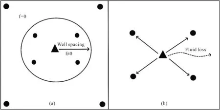
Fig.3.Schematic representation of (a) well spacing and (b) fluid loss.
2.2.Real field
On field Y(Fig.4),located in the West Kazakhstan region,there is a well stock in the amount of 70 wells that operate with high water cut (more than 80%).To understand the source of the produced water and the connectivity between injectors and producers,a tracer test was carried out in some injectors.
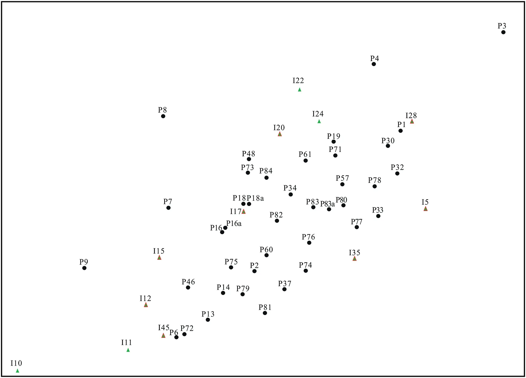
Fig.4.The location of the injection and production wells for field Y,West Kazakhstan region.
In this field,a given volume of a labeled liquid was injected and pushed back to the production wells by a continuous displacing waterflooding.Simultaneously,sampling is started from the production wellhead.Selected samples are analyzed under laboratory conditions to determine the tracer's presence and concentration.The observed tracer concentration versus time at each producer was analyzed to evaluate the influence of the water flooding on the producing wells.Environmentally friendly water-soluble sodium fluorescein and ammonium nitrate chemical agents were selected for each injection well.These agents do not affect the properties of the flow and do not chemically interact with oil.The distance from injection wells to production wells ranges from 550 m to 1300 m.By the time of testing,tracer studies were carried out within 9 days.The tracer agent was injected through two injection wells (11 and 22).18 wells were selected as control wells(wells 13,14,19,30,32,34,37,46,48,57,61,71,72,73,75,79,81,84) as shown in Fig.5.

Fig.5.Observations wells for tracer test.Red circles represent the depth of investigation.Blue circles indicate examined wells by the tracer.
3.Results and discussion
This section presents the results of interwell connectivity for the synthetic model and real field.
3.1.Synthetic model
Different scenarios were considered to investigate the effect of well spacing on interwell connectivity for the synthetic model by CRM.Fig.6 shows different well spacing scenarios for each injector.Interwell connectivity is assumed to be zero (fij=0) for the producers out of the well spacing area.There is no fluid loss associated with the synthetic model,so the summation of the interwell connectivities is equal to 1 (Σfij=1).Hence,different modeling cases are:

Fig.6.Well spacing for the synthetic field: (a) well spacing for INJ1;(b) well spacing for INJ2;(c) well spacing for INJ3;(d) well spacing for INJ4.
Case 1 -fij≠0 for the wells that are located in area 1;
Case 2 -fij≠0 for the wells that are located in area 1 or 2;
Case 3 -fij≠0 for all operating wells in the reservoir.
3.1.1.Case 1
The assumptions a) Σf=1and b)fij≠0were applied for the wells that are located inside area 1.Fig.7(a-g) show actual and estimated production rates for production wells.Interwell connectivity(fij)values are estimated by CRM,as shown in Table 1.The average simulation error is about 31%,which is almost high.This is since neglecting the connectivity between some wells can bring low accuracy to the CRM calculations.Based on the observed results,it is believed that the wells located outside of area 1 can significantly affect the performance of the wells inside area 1.
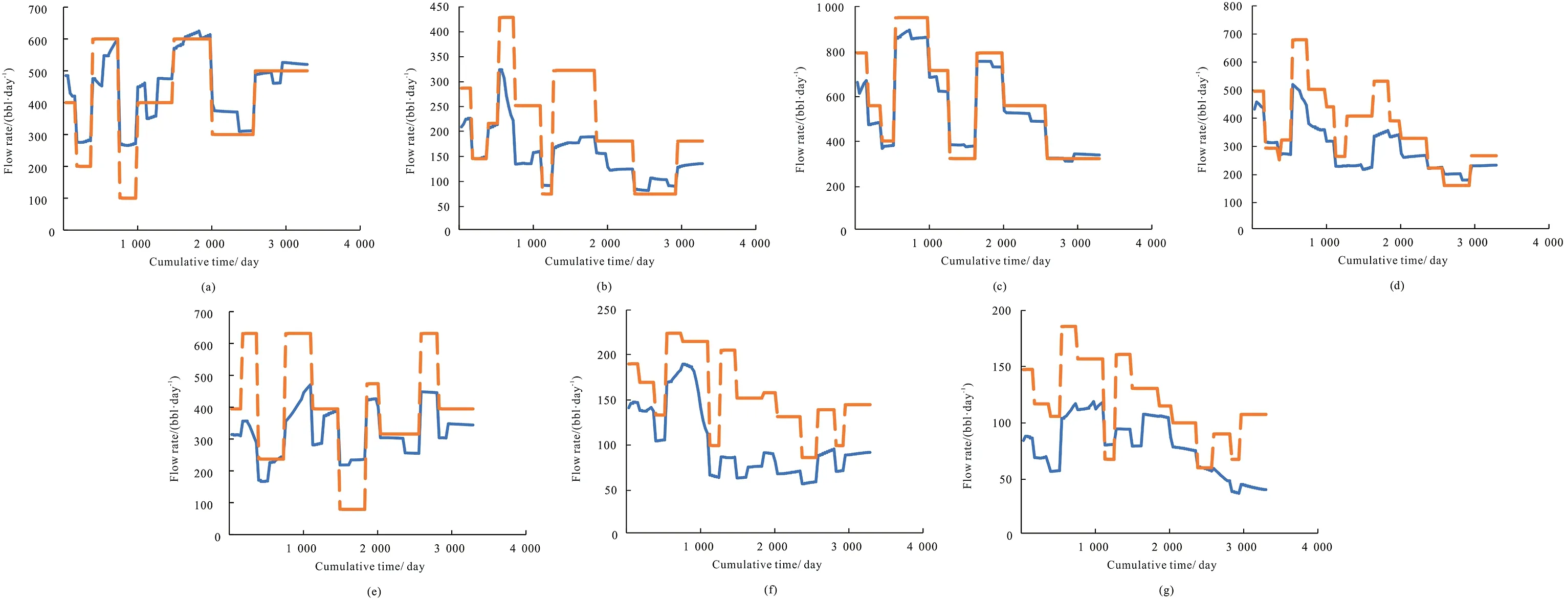
Fig.7.Example of actual production rate vs.estimated production rate: the solid blue line shows the actual production,and the dash orange line shows the production profile modeled by CRM for Case 1 (a): producer 1,(b): producer 2,(c): producer 3,(d): producer 4,(e): producer 5,(f): producer 6,(g): producer 7).
To dive deeper into the interwell connectivity between injection-production wells,we present the breakthrough time of the tracer stream for the INJ2-PRO2 and INJ2-PRO7 in Fig.8(a and b) as an example.It can be seen that breakthrough happens at different times for different pair of injection-production wells due to heterogeneity and different production schemes of the synthetic model.Breakthrough times were observed to be for PRO2 at 546 days.Producer 7 behaves differently,as the actual breakthrough happens at 1795 days,but it is a small amount of tracer agent.The clear tracer breakthrough happens 2500 days.It is believed that the earlier the tracer breakthrough,the more robust connectivity between the well pairs.Therefore,there is a stronger interwell connectivity between the INJ2-PRO2,which confirms the results of CRM (see Table 1).

Fig.8.Tracer response in the (a) producer 2 and (b) producer 7 due to injector 2.The blue line shows the tracer gain rate,and the orange line shows the tracer injection rate.

Table 2 Interwell connectivity for Case 2.
Although the tracer breakthrough time confirms the results of the interwell connectivity of CRM,there is no quantitive value for the tracer test to compare both methods.To bring the results of interwell connectivity by the tracer to a level of comparison with the results of interwell connectivity by CRM,the concept of breakthrough dimensionless number (BDN)is introduced,as presented in equation (7).
whereBDNis the breakthrough dimensionless number andshows the tracer breakthrough time for producerj.As tracerbreakthrough time is a quantitative representative of connectivity,BDNis able to make tracer breakthrough time with interwell connectivity estimated by CRM.

Table 3 Interwell connectivity for Case 3.
Hence,connectivity values were estimated by CRM and tracer tests.These values are compared as shown in Fig.9.Fig.8 justifies the trend that earlier water breakthrough leads to higher interwell connectivity.The outliers presented in these graphs happened because of the high average simulation error for this case.
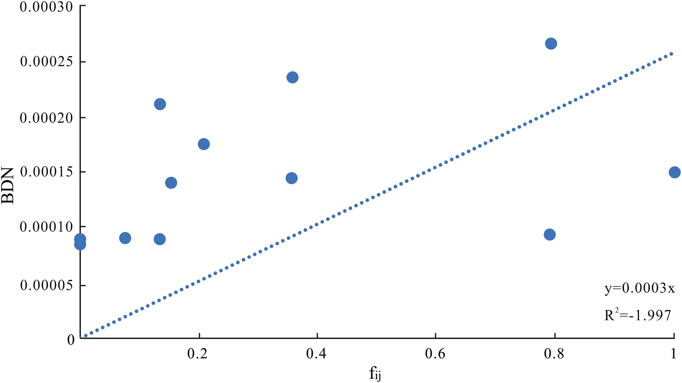
Fig.9.Comparison of interwell connectivity estimated by CRM and by tracer tests for Case 1.
3.1.2.Case 2
In this case,it is assumed that Σf=1andfij≠0for the wells located inside areas 1 and 2.Considering the well spacing,it can be noticed from Fig.10(a-i)that the CRM modeling is more accurate,and the average simulation error is reduced to about 12%compared to Case 1.fijvalues are estimated by CRM and shown in Table 2(see Fig.11).

Fig.10.Actual production rate vs.estimated production rate:solid blue line shows the actual production,and the dashed orange line shows the production profile modeled by CRM for Case 2 (a): producer 1,(b): producer 2,(c): producer 3,(d): producer 4,(e): producer 5,(f): producer 6,(g): producer 7,(h): producer 8,(i): producer 9).

Fig.11.Comparison of interwell connectivity estimated by CRM and by tracer tests for Case 2.
The higher BDN,the stronger connectivity between the wells,which can be observed by the trend of the line.Still,there is a noticeable error in the modeling,and the application of CRM is not very accurate.
3.1.3.Case 3
The same restriction was applied to Case 3,Σf=1,but for the whole field.The error of the simulation by CRM is low and about 4%in this case,as all well pair connections were considered in the model(see Fig.12(a-i)).fijvalues are estimated by CRM and shown in Table 3.
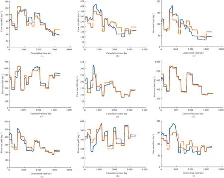
Fig.12.Example of the actual production rate vs.estimated production rate:solid blue line shows the actual production,and the dashed orange line shows the production profile modeled by CRM for Case 3 (a): producer 1,(b): producer 2,(c): producer 3,(d): producer 4,(e): producer 5,(f): producer 6,(g): producer 7,(h): producer 8,(i): producer 9).
Fig.13 shows the comparison between the two methods for Case 3.This CRM estimation is in better agreement with the connectivity results obtained by tracer test analysis due to the contribution of all wells.However,this case still has mismatches due to not accounting for fluid cross-flows.So,CRM can provide a general picture of the field's interwell connectivity and estimate the injector/producer wells with very high and very low connectivity.

Fig.13.Comparison of interwell connectivity estimated by CRM and by tracer tests for Case 3.
3.2.Real field
The tracer was injected from I11 and I22.It was gained by control wells that are circled in Fig.5.It was discovered that injection well I11 had an interwell connection that ran in the southwesterly direction of the area.An increase in the tracer agent mass transfer was observed in the zone with permeability of 115.7 mD-704.9 mD(based on the permeability filtering systems)compared to other contributing zones.Additionally,tracer agent concentrations in unplanned wells have been discovered,providing evidence of a hydrodynamic connection between injection wells and all production wells.
In order to determine the interwell connectivity betweeninjectors and producers,different scenarios were modeled by CRM.The well spacing was changed for the injectors,and different possibilities of Σfijwere also considered.By analyzing all cases,it was found that due to the presence of an active aquifer,Σfshould be greater than one.Also,well spacing should be assigned to each well.As the best scenario,Σf=1.25 for fluid loss considerations and well spacing were set as 1300 m for I11 and 950 m for I22 to contain all observation wells,as shown in Fig.5.
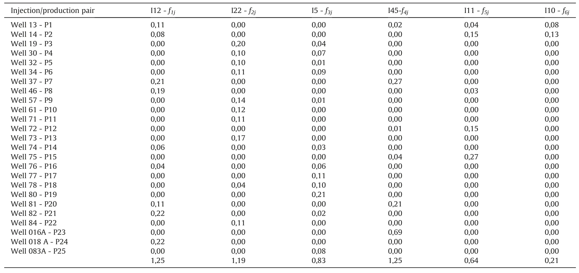
Table 4 Interwell connectivity for the real case.
History for 25 production and 6 injection wells from 01/01/2008 to 06/01/2017 was available.From 01/01/2008 to 11/01/2014 was selected as input data since there is more complete information on production and injection rates in this interval.After pre-processing the data,the CRM was applied to model the history,as shown in Fig.14.Good agreement of the calculated production with the history was observed.The average simulation error for control wells is 15%.fijvalues are estimated by CRM and shown in Table 4.Additionally,Table 4 shows the effect of fluid loss/gain.The possibility of fluid loss for injectors can be analyzed by f parameters.For example,it is estimated that I11 has serious fluid loss(Σfij=0.64).

Fig.14.Total production matching by CRM for the real field;blue-actual production,red-estimated production(a):producer 1,(b):producer 2,(c):producer 3,(d):producer 4,(e):producer 5,(f):producer 6,(g):producer 7,(h):producer 8,(i):producer 9,(j):producer 10,(k):producer 11,(l):producer 12.(m):producer 13,(n):producer 14,(o):producer 15,(p): producer 16).
These two figures presented below give a general insight into connectivities obtained from both the CRM and tracer tests.Fig.15 shows that six wells have mostly similar interwell connectivities obtained from the CRM and tracer test,and one well shows a higher value.According to Fig.16,the interwell connectivities for the wells adjacent to the injection well I11 still have problems and are very different from the data obtained by the service company.It was estimated that I11 has a severe fluid loss in this zone.This fact may be the critical factor in the significant difference between the data.An overall picture of fluid behavior in porous media may still be obtained from the CRM even when it seems that particular wells are not connected when they are in reality connected.This is because the CRM indicates the lack of connections between certain wells when they are in fact connected.
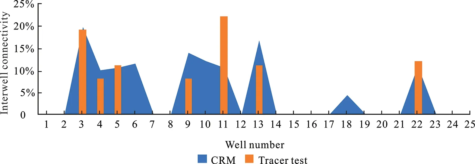
Fig.15.CRM vs.Tracer test interwell connectivities comparison for I22.

Fig.16.CRM vs.tracer test interwell connectivities comparison for I11.
Furthermore,according to the field's service company,there are difficulties with the filtration system in the northeast direction from the injection well I11,and CRM revealed somewhat abnormally high values in the same zone as the problems with the filtration system.This may imply that CRM may also describe challenges that are comparable to these.Such an approach may serve as a good precursor for actual tracer test analysis on the field and help create the tracer flooding strategies,giving the initial idea of the fluid behavior in porous media.
4.Conclusions
In this research,the capacitance-resistance model:single tank representation (CRMT) was implemented in synthetic and real fields.Different cases were tried to estimate which one could better describe the physical meaning of the interwell connectivity under certain assumptions.Such assumptions as fluid loss and well spacing were considered while mimicking the tracer field analysis.These assumptions led to different restrictions that were tried to identify the possible path of the fluids between wells.
The following ideas can be summarized:
(1) The well spacing is a critical restriction that mimics the tracer study and helps to isolate unnecessary wells and also reduces the number of unknowns;
(2) Fluid loss is also an important parameter that should be taken into consideration while working with isolating some wells from another in order to check for fluid cross-flowing from well to well;
(3) The earlier breakthrough led to stronger interwell connectivity values,which were justified by the examples of two fields;
(4) Although in some cases,the CRM shows better total production matching,interwell connectivities differ from the actual tracer results and cannot capture the physical behavior of the injected fluid.
Summing up,it can be noted the importance and necessity of introducing well spacing and fluid loss parameters to determine interwell connectivity.This approach has a significant advantage in that it mimics tracer analysis,during which only certain wells are selected for testing,and also has the physical meaning that the earlier breakthrough occurs,the higher the interwell connectivity.Considering all of the above,it can be concluded that in certain situations with properly selected constraints,the CRM can be considered a replacement for tracer testing for rapid field analysis.
Declaration of competing interest
We confirm that there is no conflict of interest in our submitted publication and our research.

- Petroleum的其它文章
- Super gas wet and gas wet rock surface: State of the art evaluation through contact angle analysis
- Petroleum system analysis-conjoined 3D-static reservoir modeling in a 3-way and 4-way dip closure setting: Insights into petroleum geology of fluvio-marine deposits at BED-2 Field (Western Desert,Egypt)
- Development and performance evaluation of a high temperature resistant,internal rigid,and external flexible plugging agent for waterbased drilling fluids
- Anti-drilling ability of Ziliujing conglomerate formation in Western Sichuan Basin of China
- Production optimization under waterflooding with long short-term memory and metaheuristic algorithm
- Experimental study on sand production and coupling response of silty hydrate reservoir with different contents of fine clay during depressurization