
Cosserat Dynamic Modeling and Simulation of Mobile Cable on Satellite
2024-01-12 13:04ZiquanWangJinzhuLiWeinanChenXuefengGaoYouLeijieShenHaojieChen
Ziquan Wang, Jinzhu Li, Weinan Chen, Xuefeng Gao, You Lü, Leijie Shen, Haojie Chen
Abstract: Mainly for the problems that the configuration of the mobile cable on the satellite is very easy to change, the motion trajectory and dynamic characteristics of the cable can not be accurately predicted, which affects the laying quality seriously, the dynamic modeling and simulation of mobile cable on the satellite are carried out.On the basis of referring to the previous papers, the existing mathematical model is improved.The equations of the base vector of the cable section principal axis coordinate system with respect to the arc coordinate s, the distribution force of cable balance equation, the matrix expression of the base vector after the rotation motion transformation in the section principal axis coordinate system, the angular velocity of cable, the section elastic strain and velocity calculation equations are given, and the Cosserat dynamic modeling of the mobile cable is established.Finally, the dynamic simulation model of the mobile cable assembly of the kinematic mechanism is established, and the changes of the force and torque on the cable constraint end are obtained, which provides a reference for the dynamic modeling and simulation of the mobile cable on satellite.
Keywords: flexible cable; large deformation; curve geometry; Cosserat modeling; computer simulation
1 Introduction
The mobile cables on the satellite mainly include the mobile cables on the motion mechanism, the mobile cables during the satellite assembly process, and the mobile cables on the moving parts in the aerospace environment.Among them, the satellite motion mechanism is a component that provides motion and bearing for satellite loads such as data transmission antenna, relay antenna, synthetic aperture radar, etc.A variety of movable cables are bundled and laid on it,including power supply cables, signal cables, etc.At present, the assembly process of satellite mobile cables mainly relies on past experience to lay, bind and fix, and following the process of design, making prototype or actual physical model, motion test, improving design, preliminarily bind and fix the prototype or actual physical model of mobile cables to the accessories of mobile structures, conduct motion polarity or launch test on mobile structures, and observe the motion state of mobile cables, record the cable movement process by camera shooting or video recording.During the movement of the mechanism, if the cable has friction interference and collision with the moving mechanism, excessive bending, excessive interference torque and other phenomena, the moving cable shall be reassembled, bundled and fixed after the motion test,and the process shall be iterated step by step to ensure that the moving cable does not have friction interference and collision with the mechanism, and the bending radius and interference torque meet the requirements of motion.During the satellite assembly process, the mobile cables include the free moving cables during the satellite side panel enclosure process and the blind area mobile cables that cannot be observed by the operator.The laying process is still faced with difficulties such as the moving cables of the moving mechanism, especially the blind area,which are invisible and unpredictable during the assembly process, and are prone to excessive bending, resulting in the cables being physically forced to be assembled, even damaged or broken by pulling or pressing.The mobile cables on the moving parts in the aerospace environment mainly refer to that the cables installed on the satellites are forced to follow the movement because of some products, such as optical lenses,detectors, etc.In summary, it can be seen that due to the fact that mobile cables are very easy to change their configuration when laying, some cables are located in unobservable cabin sections in the blind area, the previous cable design and test interaction is frequent and the cycle is too long, and the motion trajectory and dynamic characteristics of cables during the deployment of mechanisms, satellite assembly, and component activities cannot be accurately predicted, which makes it difficult to comprehensively assess and avoid the risks after laying, and seriously affects the quality of cable laying.At present, excellent 3D CAD software such as Pro/E, CATIA, and SolidWorks are used for the cable design [1-4],but the software only carries out cable layout and configuration design based on spline curve without considering the actual physical parameters such as cable density, tensile bending stiffness, elastic modulus, shear modulus and moment of inertia, as well as the external gravity environment and distributed contact force environment in which the cable is located, The authenticity and accuracy of the cable design results are poor.Therefore, it is necessary to study the dynamic model of satellite cables, especially mobile cables,which considering physical characteristic parameters.
In terms of physical characteristics, cables can be compared to elastic slender beams.Therefore, the dynamic theory course for elastic slender beams should be applied to the dynamic modeling of cable.At present, more and more scholars at home and abroad have studied the application of elastic thin rod dynamics in engineering [5-10].The dynamic analogy method proposed by Kirchhoff in the year of 1859 converts the deformation of the elastic rod into the rotation of the rod section along the rod centerline[11-15], so that the statics of the elastic rod has the same mathematical expression as the dynamics of the rigid body, and only the time variabletis replaced by the arc coordinates[16-20].After adding inertial force and time variables, it can be used for dynamic modeling of elastic rod, and has also been used in the dynamic modeling of large deformation beams in engineering [21-23].When considering the shear and tensile deformation of the cable section, the Cosserat dynamic modeling is more suitable for the elastic thin rods.Mobile cables on the satellite have the characteristics of complex environment within the scope of activity, multiple coupling assemblies, frequent interference and collision with stars, surrounding single machines, cables and other products.Therefore, the core issue of dynamic simulation for mobile cables on the satellite is rapid dynamic simulation of assembly contact and collision.
On the basis of referring to the previous papers, this paper carries out the geometric modeling and detailed derivation of the flexible cable.According to the analysis of the curve geometric model, the equations of each dimension of the cable section principal axis coordinate system with respect to the arc coordinatesare given.Considering the distributed force elements on the center line of the actual cable physical model, the belt force balance equation is given.According to the Kardan angle transformation of the shear deformation of cable section, the matrix expression of the base vector after the centerline transformation caused by the shear deformation in the coordinate system without shear deformation is given, and the calculation equations of the cable deflection and angular velocity matrix are given.The micro arc deformation of cable is analyzed,and the calculation formulas of elastic strain and velocity of the cable section are given.Finally,the Cosserat dynamic modeling of mobile cable is carried out, which provides the theoretical basis for the motion and dynamic calculation and simulation of flexible cable.
2 The Geometry Model of Cable
2.1 The Geometry Model of Curve
The basic theory of elastic thin rod dynamic model is curve geometry.A spatial smooth curveCwith length ofLis shown in Fig.1.TheP0on the curve is the origin point, and the arc coordinatesof the curve is established under the condition that the curve has no telescopic deformation.At the same time, the fixed coordinate systemO-ξηζis established with the fixed origin pointOin space, and its base vectors areeξ,eη,eζ.Then the arbitrary pointPon the curve can be determined by the arc coordinatesand the vector diameterrrelative to the fixed pointO.ris the vector that completely determines the geometry of curveCand the single value continuous differentiable function about the arc coordinates.Then the tangent direction unit vector of curveCat pointPis
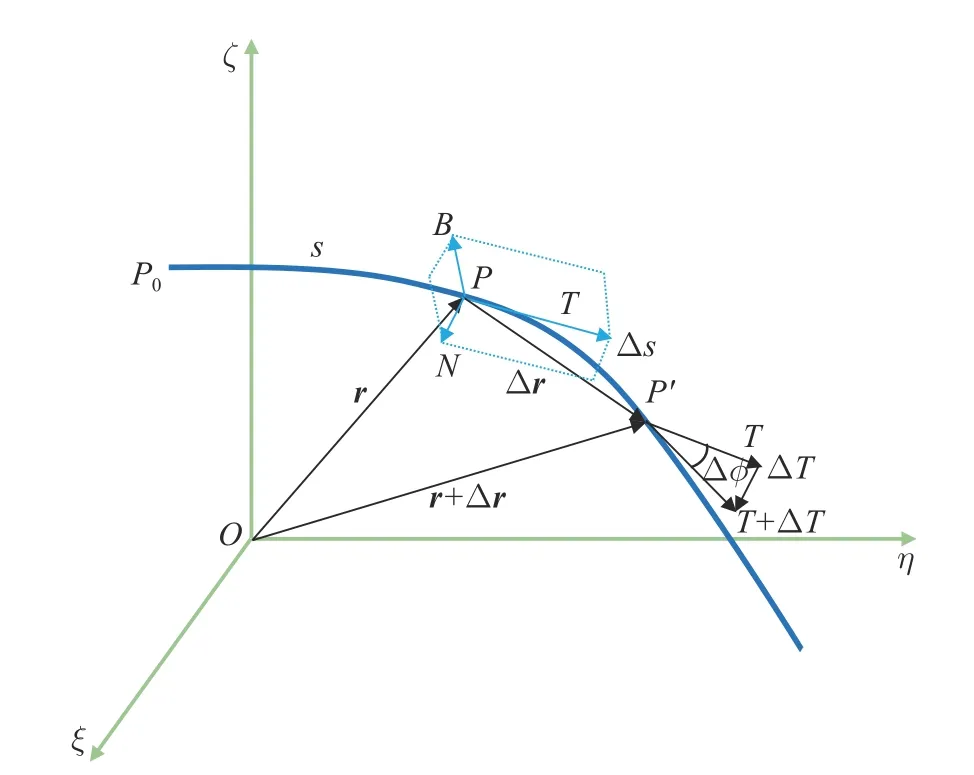
Fig.1 Infinitesimal angular displacement and the Frenet coordinates of spatial smooth curve
The modulus of derivative of theT(s) onsis defined as the curvature of curveCat pointP,and the expression is
Define the infinitesimal angular displacement when pointPon curveCmoving to the adjacent pointP′as Δ?.When Δs →0, the curvature expression is
Therefore, curvature is a parameter to measure the degree of curve bending, and its reciprocal is called the radius of curvature
The unit vector along the direction dT/dsis called the normal vector of curveCat pointP,which is recorded as
According to the right-hand spiral rule of the coordinate system, the sub-normal vector of curveCat pointPis recorded as
In Fig.1, the coordinate system composed ofP-NBTis the Frenet coordinate system, and its base vectorsen,eb,etare equal toN,B,T.The plane formed byTandNis the osculating plane,and the plane formed byNandBis the normal plane.Suppose pointPmoves in the positive direction of arc coordinatesat unit speed along curveC, then the rotation angular velocity of the normal plane around axisBisκ(s), and the rotation angular velocity vector of the osculating plane around axisTis
The modulus ofτ(s) is called the torsion of curveCat pointP, so the rotational angular velocity of the Frenet coordinate system relative to the fixed coordinate systemO-ξηζis
According to Eq.(1) to Eq.(8), the equations of each dimension of Frenet coordinate system with respect to the arc coordinatescan be obtained
Then the position of the space curveCrelative to the fixed coordinate system can be obtained from the following equation as
In Eq.(10),σis the integral variable, andr(0) represents the spatial position of pointP0.According to Eq.(8) to Eq.(10), curvature and torsion are two independent variables to determine the spatial curve.Therefore, it can be seen that the freedom degree of the spatial curve is 2.
2.2 The Geometric Bending and Torsion of Cable
As shown in Fig.2, the section principal axis coordinate systemP-xyzrotates a torsion angle around the axis ofTrelative to the Frenet coordinate system.The base vectors of the section principal axis coordinate systemP-xyzaree1,e2,e3.It can be obtained that the angular velocity vector of the cable section relative to the fixed coordinate systemO-ξηζis

Fig.2 The Frenet coordinate system and the principal axis coordinate system of the cable section
It is knowable thatωis the vector of cable bending and torsional deformation, which is called bending and torsion degree, and the three components of bending and torsion degreeωi(i=1, 2, 3) are the three independent variables that determine the geometric form.Similarly,other coordinate systemsP-d1(s)td2(s)td3(s)twhose origin is the pointPcan also be associated with coordinate rotation.
From the coordinate change relationship, the equations of each dimension ofP-xyzcoordinate system with respect to arc coordinatescan be obtained
3 Distribution Force Balance Equation of Cable
Considering the possible contact or mutual contact between cables and other objects, there must be a distributed contact force.If the electrostatic effect between cables is considered, the distributed electrostatic attraction must be introduced.When discussing the movement of cables in viscous medium, the viscous resistance and moment must also be introduced.Therefore, the balance equation should take the distributed force and moment into account.
As shown in Fig.3, the force balance diagram ofP-P′micro arc section under distributed force, gravity and gravity moment.In the figure,Mis the moment,Fis the force,fandmare the distributed force and moment,fgandmgare the gravity, and gravity moment,respectively.It can be seen that the resultant force and resultant moment at pointPare zero in the equilibrium state, that is

It should be pointed out that if the friction or tangential gravity is not considered, the forcef3=0.If the distributed forces are omitted, the equation will become the equilibrium equations without scoring the distributed forces.The distributed moment appears only when moving in a viscous medium, so it can be omitted in the discussion of statics.

Fig.3 Distributed force balance of cable micro arc section
Since the cables on the satellite are in the power-off state when laying or moving, the electrostatic attraction between cables can be ignored.The viscosity coefficient of air is very small, so the viscous resistance of the cable moving in the air can also be ignored.However, due to the existence of earth gravity and cable indirect contact force, the distributed force on the cable can not be ignored.
4 Dynamic Model of Cable
4.1 Angle Transformation of Kardan with Shear Deformation
Before making the Kardan angle transformation,it is necessary to point out the section deformation as follows.
1) Geometric characteristics: The cable has certain quality and deformability; Compared with the cross-sectional size, the cable is much larger in length and radius of curvature; Due to the bending and torsion of the cable itself, the two sections of the same cable micro section can rotate relative to the center line.
2) Physical properties: Take the cable with circular section, the material is homogeneous and isotropic, and the stress and strain meet the linear constitutive relationship; The cross section of the cable end is regarded as a rigid plane that cannot be deformed.
As shown in Fig.4, the cable section attitude is described using the Kardan angle coordinate transformation system.The Kardan angle transformation needs to consider four groups of coordinate systems:O-ξηζ(fixed coordinate system),P-xyz( section principal axis coordinate system),P-x0y0z0(transition coordinate system)andP-xsyszs( section normal and section fixed coordinate system).Moving the originOof the coordinate system to the pointPon the cable in the figure,ψis the rotation angle around theξaxis from the coordinate systemP-x0y0z0;θis the rotation angle ofP-x0y0z0around the axisy0to the coordinate systemP-xyz, where thez-axis is the normal axis of the section;φrefers to the rotation angle ofP-xyzaround thez-axis, to the coordinate systemP-xsyszs, and fixed with the section,the Kardan angleψ,θ,φdetermine the attitude of the section after rotation.

Fig.4 Angle transformation of Kardan
Takee3as the base vector, the section has no strain in theO-xyplane, and an infinitesimal rotation vectorδis generated in the center of the section in theO-xzandO-yzplanes to the coordinate systemP-x*y*z*, where thez*-axis direction is along the tangent direction of the centerline, as shown in Fig.5.Note that the strain in theP-xyzcoordinate system isε1=δ13,ε2=-δ23, then the projection ofδin theP-xyzcoordinate system is
Thez*-axis of the coordinate systemP-x*y*z*is the position after the rotation of thez-axis ofP-xyz.The base vectore*is expressed inP-xyz.Taylor expansion is carried out for small variablesδ13,δ23, and the quadratic small quantity is ignored.The expression of the base vectore*inP-xyzis as follows

Fig.5 Centerline rotation transformation
Eq.(18) is the matrix expression of the base vector transformed by the centerline caused by shear deformation in the coordinate system without shear deformation.
Let the matrixAbe the rotation matrix of the rigid body around the local rectangular coordinate system.According to the rotation kinematics of the coordinate system, we can get
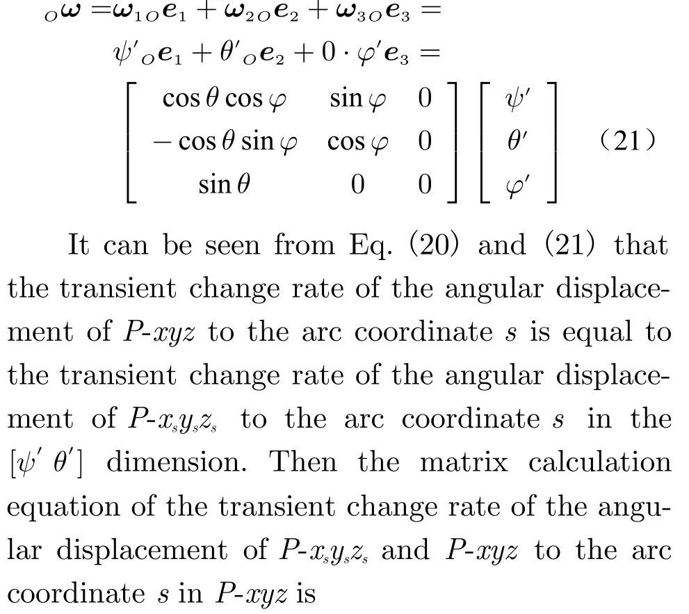
Let the transient rate of change of the angular displacement ofP-xyzto the arc coordinatesand timetbe recorded asωandΩ, the transient change rate of the angular displacement ofPxsyszsto the arc coordinatesand timetis recorded asωsandΩs, note thatω′is the derivative of angular displacement to arc coordinatesand Ω˙ is the derivative of angular displacement at timet.The expression of the transient change rate of angular displacement ofP-xsyszsto the arc coordinatesinO-ξηζis
The expression of the transient change rate of the angular displacement ofP-xyzto the arc coordinatesinO-ξηζis

Similarly, it can be obtained that the transient change rate of angular displacement ofPxsyszsandP-xyzat timetis expressed inP-xyzas
The principle of micro-arc deformation of cable which is shown in Fig.6.In order to understand the deformation principle of the cable micro arc segment, the basic vectore3of the section principal axis coordinate system and thezdirection elastic strain are added to the micro arc segment deformation bodyε3, the cable section shows tensile deformation when moving along thez-axis; when rotating around thez-axis, it shows torsional deformation.When moving along the axis ofxory, it shows shear deformation.When rotating around the axis ofxory, it shows the bending deformation.
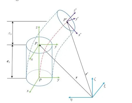
Fig.6 Micro arc deformation and strain along z-direction
Before the elastic deformation of the cable,take the micro arc segment Δsandr(s,t) along the center line of pointPas the vector diameter of pointPrelative to the fixed pointO, we can get
Then the partial derivative of vector diameterronsis
Consider the vector diameter after deformationr*(s,t), and setε1,ε2,ε3are the projection of the deformed strain onP-xyz, we can get
From Eq.(27) to Eq.(29) , it can be obtained
The representation of the component of the vector diameterr*in the fixed coordinate is recorded asξ(s),η(s),ζ(s), the representation of the vector diameterr(0)in the fixed coordinate is recorded asξ0(s),η0(s),ζ0(s), and the displacement due to the shear deformation and expansion deformation of the body of the section is recorded asw(s,t), then we get

According to Eq.(24) and Eq.(32), we can get

The Eq.(38) is the strain matrix after considering shear and tensile deformation.It can be seen that the strain matrix of the cable section is related to the displacementw, Kardan angleψ,θand initial Kardan angleψ(0),θ(0)caused by telescopic deformation.Convert the arc coordinatesinto timetaccording to Eq.(26), Eq.(32), and Eq.(38), the expression of the speed of the cable section in theP-xyzcoordinate system is expressed as
It can be seen thatψ,θ,φ,w1,w2,w3are the six generalized coordinates to determine the cable configuration, and the bending torsion, the section angular velocity, elastic strain, and velocity parameters of the rod can be determined by the derivatives of these six generalized coordinates to the arc coordinatesand timet.
4.2 Dynamic Model of Cable
Define the cable shear stiffness coefficient asK;The tensile stiffness coefficient isK0; the bending stiffness of the section around thex-axis isA(A=EIx),Eis the elastic modulus, andIxis the moment of inertia of the section relative to thexaxis; the bending stiffness of the section around they-axis isB(B=EIy), andIyis the moment of inertia of the section relative to they-axis; The torsional stiffness of the section around thez-axis isC(C=GIz),Gis the cable shear modulus, andIzis the polar moment of inertia of the section relative to thez-axis;ρis the density of the cable;Sis the cross-sectional area of the cable;Jis the inertia tensor of per unit length of cable;The bending and torsion of the cable in the initial state is
Then the projection of forces and moments on the coordinate systemP-xyzis
According to the momentum theorem and momentum moment theorem of Newtonian mechanics, the cable dynamics model can be obtained as follows
Let the moment of inertia ofJalong the axes ofxandybeρI.Then the moment of inertia along thez-axis is 2ρI.SetJ0andIas the moment of inertia of the section.Consider the cable with circular section, we can get
Thus

The Eq.(48) is the Cosserat dynamic model mobile cable.Bring Eq.(38), Eq.(39), and Eq.(41) into Eq.(48) to obtain the closed equations ofψ,θ,φ,w1,w2,w3, which can be solved by numerical integration method.
The Ref.[22] and Ref.[23] established the cable dynamic model based on the accurate Cosserat elastic rod model, which is more suitable for the dynamic modeling of large deformation cables in engineering.The modeling methods in the two articles are essentially the same,so they relatively obtained a similar dynamic equations, but the equations of arc coordinatessin each dimension of the cable section principal axis coordinate systemP-xyzdue to the change of coordinates, and the expression of infinitesimal rotation basis vector generated by the section center inP-xyzare not derived.According to the force analysis of micro element, the Ref.[22]gives the correct unified equation for the partial differential calculation of force and moment,which provides a theoretical basis for the cable dynamics modeling.However, the third term of the moment partial differential equation of formula (19f) in Ref.[22] has an independent item angleθ.The independent term ofθand the lack of force and strain action components are also reflected in Ref.[23].In this paper, the Eq.(48)proved that the angleθshould appear in the form ofθ′, that is in the form of the first derivative of the arc coordinates.At the same time,the force and strain components are added in the Eq.(48).
5 Flexible Cable Simulation of Deployment Mechanism
The numerical method of adaptive step-size can be used to calculate the differential equations, so as to realize the rapid dynamic simulation of satellite mobile cable of assembly contact and collision.Set the physical parameters of cable as shown in Tab.1.
The three-dimensional simulation model of the flexible cable of the deployment mechanism is established, as shown in Fig.7.In the figure, the deployment mechanism and flexible cable model are simply simulated, the model includes a fixed part (fixed pair with the ground), a rotating part(rotating pair with the ground, the rotation center is the pointOin the figure, and the rotation axis isz), and a flexible cable with physical properties as shown in Tab.1.The connection between one end of the cable and the fixed part is a fixed connection, and the connection between the other end of the cable and the rotating part is a fixed connection, but it can follow the movement with the movement of the rotating part.Set the rotation speed of the rotating part around thez-axis to 1(°)/s, ignore the effects of gravity, set the total simulation time is 90s, and the simulation step size is 1s.

Tab.1 Simulation parameters of cable

Fig.7 Simulation model of deployment mechanism cable
The following movement of the flexible cable is obtained, as shown in Fig.8.It can be seen that the fixed end of the flexible cable remains fixed with the earth during the movement of the rotating part; the mobile fixed end follows the movement of the rotating part, and achieves a good simulation effect.The cable changes from the initial relatively relaxed state to the tensioned state gradually, and there is a transitional bending and torsion phenomenon at the fixed end, which indicates that the cable will be subjected to large force and torque.It is necessary to increase the cable length to ensure that the cable remains relatively relaxed during the movement of rotating parts.It can be further demonstrated from the changes of forces and torques on the cable.

Fig.8 Following motion of flexible cable of deployment mechanism
The force variation curves of the fixed end and the mobile fixed end of the cable are obtained, as shown in Fig.9.It can be seen that the resultant force on the fixed end increases with the movement of the rotating part gradually, and the maximum value of the resultant force is 1 319 N, in which the force in thexdirection changes in a semi elliptical shape, while the force in theydirection changes in a quarter elliptical shape, which is related to the rotating part rotating around thez-axis, symmetrical in thexdirection and asymmetric in theydirection,which is in line with the actual situation.The force of the resultant force on the fixed end of the cable in thezdirection is almost zero, which is related to the non-gravity distribution force in the simulation environment, which is in line with the actual situation.The resultant force on the moving fixed end gradually increases with the movement of the rotating part, and the maximum value of the resultant force is 1 319 N.Its component force in thex,y,zdirection is almost the same as that of the fixed end resultant force in thex,y,zdirection, and the direction is opposite.It can be seen that the resultant force of the two constraint ends on the cable is almost zero,which is related to the fact that the deployment mechanism is only provided with rotational motion.

Fig.9 Force change of fixed end and mobile fixed end of flexible cable: (a) force change of fixed end; (b) force change of mobile fixed end
The resultant force on the moving fixed end gradually increases with the movement of the rotating part, and the maximum value of the resultant force is 1 319 N.Its component force in thex,y,zdirection is almost the same as that of the fixed end resultant force in thex,y,zdirection, and the direction is opposite.It can be seen that the resultant force of the two constraint ends on the cable is almost 0, which is related to the fact that the deployment mechanism is only provided with rotational motion.
The variation curve of the resultant moment of the fixed end and the mobile fixed end of the cable is obtained, as shown in Fig.10.It can be seen that the resultant moment of the fixed end gradually increases with the movement of the rotating part, reaching the maximum value at about 78 s, with the maximum value of 5.25 N·m.the torque value decreases in 78 s-90 s.The moment at the mobile fixed end shows an approximate semi-elliptical variation trend,reaching the maximum value at about 35 s, and the maximum value is 0.69 N·m.Since the fixed end does not move with the rotating part, but produces large bending and torsional deformation with the movement of the rotating part, the torque value at the fixed end must be greater than that at the moving fixed end, which is in line with the actual situation.
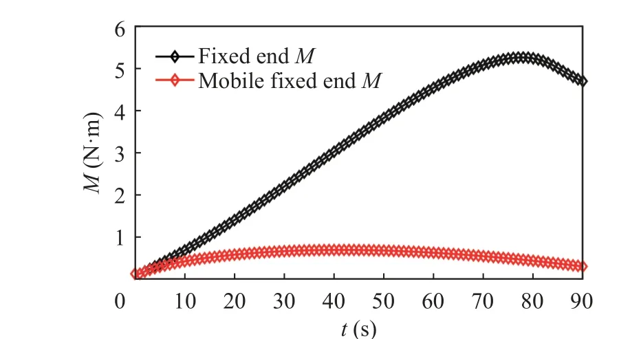
Fig.10 Variation of the resultant moment of fixed end and mobile fixed end of flexible cable
6 Conclusions
This paper can be summarized as follows.
1) The Cosserat dynamic modeling of the mobile cable is established, and the existing mathematical model is improved.According to the Kardan angular coordinate transformation system, the matrix expression of the base vector after the center line transformation caused by shear deformation in the coordinate system without shear deformation is obtained, and six generalized coordinates in the cable dynamics are obtained.From this, the angular displacement vector, elastic strain equation, and velocity equation of the outgoing cable are derived, and the Cosserat dynamic model of the cable with arbitrary circular section is obtained according to the theorem of momentum and moment of momentum, which provides a theoretical basis for the dynamic calculation and simulation of the flexible cable.
2) The three-dimensional model and simulation of the flexible cable of the deployment mechanism are carried out, the trajectory of the flexible cable following the movement of the deployment mechanism is obtained, and the changes of the force and torque at the constraint end of the cable are obtained, which provides a reference for the dynamic simulation of the flexible cable.
3) The theory and simulation of cable dynamics and some simulation results are obtained.In the subsequent research, we can use the sensors of force, displacement, and transmitter devices, etc.to measure the parameters during the cable movement, and compare them with the simulation results.At the same time, the theoretical model in this paper can be compared with other dynamic models.For cables with the same physical properties, the calculation results obtained by different theories can be observed, so as to select a more appropriate theoretical model,and to improve the theory and simulation model further.
 Journal of Beijing Institute of Technology2023年6期
- Journal of Beijing Institute of Technology的其它文章
- Nonlinear Trajectory SAR Imaging Algorithms:Overview and Experimental Comparison
- Post-Processing of InSAR Deformation Time Series Using Clustering-Based Pattern Identification
- 3D Target Localization Based on FrFT from Spaceborne Curve SAR
- Modeling and Analysis of the Impacts of Temporal-Spatial Variant Troposphere on Ground-Based SAR Imaging of Asteroids
- Analysis and Experimental Study on the Friction Force at the Binding Point of Flexible Cable on Satellite
- SAR Tomography with Improved Non-Local Means Filtering Based on Adaptive Window