Deinterleaving of radar pulse based on implicit feature

GUO Qiang, TENG Long, WU Xinliang, QI Liangang,*, and SONG Wenming

1.College of Information and Communication Engineering, Harbin Engineering University, Harbin 150001, China;2.China National Aeronautical Radio Electronics Research Institute, Shanghai 200030, China

Abstract: In the complex countermeasure environment, the pulse description words (PDWs) of the same type of multi-function radar emitters are similar in multiple dimensions.Therefore,it is difficult for conventional methods to deinterleave such emitters.In order to solve this problem, a pulse deinterleaving method based on implicit features is proposed in this paper.The proposed method introduces long short-term memory (LSTM)neural networks and statistical analysis to mine new features from similar PDW features, that is, the variation law (implicit features) of pulse sequences of different radiation sources over time.The multi-function radar emitter is deinterleaved based on the pulse sequence variation law.Statistical results show that the proposed method not only achieves satisfactory performance, but also has good robustness.

Keywords: multi-functional radars of the same type, pulse deinterleaving, pulse amplitude, implicit feature, long short-term memory (LSTM) neural networks.

1.Introduction

In the electronic reconnaissance, the mission of the electronic warfare (EW) receiver is to intercept emitter pulses of interest as much as possible.Normally, these intercepted pulses are interleaved.Pulse deinterleaving means to separate these interleaved pulses based on the pulse description word (PDW) to obtain the emitters of interest.PDW includes pulse amplitude (PA), time of arrival(TOA), pulse repetition interval (PRI), pulse width (PW),radio frequency (RF), and direction of arrival (DOA).Traditional de-interlacing methods fall into two main categories: (i) PRI-based de-interleaving methods, including the cumulative difference histogram (CDIF) algorithm[1], the sequential difference histogram (SDIF) algorithm[2,3], and the PRI transforms algorithm [4-6]; (ii) clustering methods based on multi-dimensional features (RF,PW, DOA, etc.), including support vector clustering and fuzzy clustering [7-11].The preconditions of the above methods are that the features of the same emitters have good correlation, and different emitters have good separability.In addition, there are some novel de-interleaving algorithms.For example, Liu and Yu [12] solved pulse classification, denoising, and de-interleaving problems using residual neural network (RNN).The features it used are PRI and PW.Gencol et al.[13] used PA to estimate the angular scan velocity of the radiation source, and combined PRI, PW, and DOA for clustering to accomplish pulse deinterleaving.The prerequisite for both methods is the distinguishability of PW and DOA for different emitters.

However, in a complex electromagnetic environment,the EW receiver often intercepts two or more emitter pulse sequences from the same type of radar.These pulse sequences have multiple modes, including search mode and track and search (TAS) mode [14,15].The PW and RF features of different emitter pulse sequences are basically the same.In addition, the distance between formation aircraft is much smaller than the distance between the receiver and aircraft.The accuracy of direction finding of the EW receiver is not sufficient enough to distinguish the DOA of multiple emitters.PW, RF, and DOA cannot be used for pulse deinterleaving, that is, the clustering methods fail in such circumstances.The feature parameters of the advanced complex radar system in the time domain have various changes and a large range of changes.Therefore, the PRI-based method cannot be used directly.Features that can be used for pulse deinterleaving include TOA and PA.However, there are few studies on pulse deinterleaving of emitters using TOA and PA features.There are many studies on the analysis of the variation law of PA.Under different antenna scanning types, [16-19] proved that there is a certain variation law of PA through real data and simulation data.The variation law of PA is related to the pattern of the antenna.In addition, Guo et al.[20] proposed a trajectory featurebased pulse de-interleaving method using TOA and PA.It can only solve the problem of deinterleaving search pulses in the case of overlapping air and frequency domains.

Multifunctional radar emitters have multiple modes of operation.The intercepted pulse sequences include both search and tracking pulses and are very heavily interleaved in the air, time, and frequency domains.In order to solve this problem, firstly, this paper analyzes the sequence variation law of search pulse and tracking pulse.Their variation patterns are very different and less correlated.Therefore, the variation pattern of the tracking pulses sequence (implicit feature) is extracted by statistical analysis, and the feature is used to separate the search pulses from the tracking pulses.Secondly, long shortterm memory (LSTM) neural network is used to extract the trajectory change pattern of the search pulse sequence.On this basis, the pulse envelope prediction model and the sequence trajectory tracking model are established to complete the de-interleaving of the search pulses.Then, support vector clustering (SVC) is used to classify the tracking pulses.Finally, results are obtained by fusing the above de-interleaved results based on the correlation between the search and tracking pulses of the same emitter.

The rest of this paper is organized as follows.Section 2 introduces the mathematical model of PA and the criterion of amplitude information change.In Section 3, the detailed of the proposed method is presented.Simulations are carried out in Section 4 to demonstrate the performances of the proposed methods.Section 5 concludes the paper.

2.PA model

2.1 Mathematical model

The PA can be expressed by the power density of the radar signal received by the EW receiver.The amplitude change is mainly caused by antenna beam modulation,which reflects the scanning law of the antenna.The power densityS[21] is

wherePtis the radar signalpower,Gtisthemaximum antennagain,Rrepresents the distance betweentheradar and the reconnaissance platform,Lis the electromagnetic wave transmission loss,Ft(·) is the normalized antenna pattern function, and θ is the angle between the line of sight of the reconnaissance equipment at the radar platform and radar antenna.Because the distance and the angle between the EW receiver and the emitter is considered negligible changes, the termPtGt/[(4πR)2L] is considered constant.This assumption is suitable for static combat scenarios and scenarios where the antenna scanning rate is much faster than the motion of the airborne platform, which is most common in electronic warfare.Thus,the received signal power is a function ofFt(θ).The PA in the experiment is the relative power of the signal after logarithmic amplification processing, sampling, holding and storage, the unit of PA is dB.Sis expressed in decibels:

whereGt,Ft(θ) , andLare the corresponding decibels.For the radar under tracking,Ft(θ) =1.For the radar in the search state,Ft(θ) is affected by the radar beam shape and scanning pattern.

The purpose, performance, and carrier of the radar are different, and the pattern function of the radar antenna is different.Therefore, accurate expressions of pattern function are often complicated.In order to facilitate engineering calculations, simple functions can be used for approximation, which can be represented by Gaussian function or Sinc function as follows:

where θ0.5is the -3 dB beam width.

2.2 Law of PA change

The premise of analyzing the law of amplitude information changes.The radar antenna has a certain pattern.During the radar scanning, the pattern of the antenna is shown to the reconnaissance antenna in a certain motion.The radar emitters are working in search or tracking state.In general, the radar periodically scans in a circle at a certain angular velocity, and the antenna pattern is generally represented by Gaussian function or Sinc function [16].Therefore, the above premises can be satisfied.

When the location of the reconnaissance equipment is scanned, the beams meet and the receiver detects the pulse and determines its parameter.The number of pulses in the encounter period are the number of pulses received in the periodic scan.There are two working patterns of radar: tracking pattern and searching pattern, and PA features are different under different working patterns [22].

Regardless of human interference, the amplitude of the search pulse in a single scan period is a function of the radar antenna pattern, i.e., the PA change law is similar to the Sinc function.When the relative motion between the EW receiver and the emitter is significant, the PA becomes a function of the changing distance.In the tracking state, after the radar locks the target, it continuously emits pulses to the target to achieve tracking of the target.The reconnaissance platform receives continuous pulse information, and the tracking PA is a function of the distanceRbetween the radar and the reconnaissance platform.The PA distribution features in these two patterns are shown in Fig.1(a) and Fig.1(b), respectively.However, there are inevitable PRI jitter, missing pulses, and environmental noise in the actual environment which is introduced in the experiment part.

Fig.1 PA distribution

3.Proposed method

The structure diagram of the proposed method is shown in Fig.2.First, pre-processing and trajectory feature extraction of the pulse sequence can reduce the effects of PRI jitter, pulse loss, and environmental noise to a certain extent.Since the pulse sequence includes tracking pulses and searching pulses, and the trajectory change characteristics of the two pulses are different, it is necessary to separate them apart.Then the search and tracking pulses are classified using LSTM and SVC, respectively.Finally, the classification results are fused to obtain the final de-interleaved results.Each part of the proposed method is discussed in detail below.

Fig.2 Framework of proposed method for pulse deinterleaving

3.1 Pulse sequence pre-processing

The purpose of pulse pre-processing is to reduce the influence of PRI jitter, missing pulses, and environmental noise on the changing law of pulse trajectory, to better extract trajectory features.Since the intercepted pulse sequence is overlapped, it is necessary to classify the pulse clusters to obtain non-overlapping pulse clusters and overlapping pulse clusters.Then, the pulse cluster is denoised.Finally, the idea of segmentation is used to segment each pulse cluster and extract the centroid pulse.

3.1.1 Pulse cluster classification

Typically, for phased-array radar emitters, the PA variation during the beam dwell time is small.The PA variation between different wave positions is large [13,18].Based on this, we use the first-order amplitude difference method to process the pulse sequence without distinguishing between the emitter pulse signal and the noise.The amplitude difference can be calculated as

whereNis the total number of pulses.The pulse clusters are classified according to the amplitude difference detection threshold δ?PAand the number of pulses over the detection threshold δnum.That is

According to (5), we can obtain non-overlapping clusters and overlapping pulse clusters.The above process is shown in Fig.3, where the pulse clusters in the dashed box are the overlapping pulse clusters PAol, and the others are the non-overlapping pulse clusters PAnol.

Fig.3 Sketch of the pulse cluster classification

3.1.2 Pulse cluster denoising

Since the intercepted emitter signal includes not only the pulse signal of interest but also a large amount of noise.Therefore, it is necessary to filter the clusters of nonoverlapping and overlapping pulses separately, so as to filter out most of the noise and reduce the impact on the subsequent pulse de-interleaving.Pulse cluster filtering can also use first-order amplitude differencing to filter out noise.The first-order amplitude difference of the nonoverlapping pulse cluster is

whereKis the total number of pulses in the non-overlapping pulse clusters.According to δ?PAfor the non-overlapping pulse cluster denoising, when ?PAnolk≥δ?PA, the corresponding data samples are noise, and the rest of the data samples are emitter pulse signal, noted as PAnolF.

The denoising process of the overlapping pulse cluster PAolis different.First, the first-order amplitude difference is performed on PAol.

whereLis the total number of pulses in the overlapping pulse clusters.Then, the overlapping pulse clusters are classified based on δ?PA.When ?PAoll<δ?PA, the corresponding data sample is the emitter pulse.And the data sample of ?PAoll≥δ?PAis calculated once more for the first-order amplitude difference and compared with the threshold δ?PA.The data samples larger than δ?PAare noise and the denoised overlapping pulse clusters are noted as PAolF.

3.1.3 Non-overlapping pulse clusters segmentation

First, the first pulse of PAnolFis defined as the reference pulse.Then the amplitude difference ?PAnolFis calculated sequentially starting from the second pulse.When?PAnolF≥δ?PA, the corresponding pulse, i.e.the segmentation point PAnolFmarkof the pulse cluster, is recorded.And the reference pulse is updated (the next pulse at the segmentation point).The above process is repeated to obtainZsegmentation points, corresponding toZ+1 pulse clusters.

where {·} is a cluster of pulses.The segmentation schematic is shown in the solid box in Fig.4.Finally, the centroid pulse {TOAnolFR,PAnolFR} is extracted, as shown by the black solid dots in Fig.4.

Fig.4 Schematic diagram of pulse cluster segmentation

3.1.4 Overlapping pulse clusters segmentation

First, the first pulse of P AolFis defined as reference pulse 1.And the amplitude difference ?PAolF1is calculated sequentially starting from the second pulse.When?PAolF1≥δ?PA, the corresponding pulse is recorded as the reference pulse 2.Then the amplitude difference?PAolF2of the reference pulse 2 is calculated.

When (11) is satisfied, the corresponding pulse, i.e.,the segmentation point PAolFmarkof the pulse cluster is recorded.

Reference pulse 1 and reference pulse 2 are updated simultaneously.The above process is repeated to obtainVsegmentation points, corresponding toV+1 segment pulse clusters.The segmentation schematic is shown in the dashed box in Fig.4.

Since PAolFis an overlapping pulse cluster, each {·} in PAolFcontains two pulse clusters, i.e., it needs to be processed using first-order amplitude differencing.Finally,the centroid pulse {TOAolFR,PAolFR} is extracted based on(9) and (10), as shown by the solid gray point in Fig.4.The centroid pulse {TOAnolFR,PAnolFR} with non-overlapping pulse cluster and the centroid pulse {TOAolFR,PAolFR}with overlapping pulse cluster are unified and noted as{TOAFR,PAFR}.

3.2 Extraction of trajectory feature

Based on the analysis of the trajectory variation law of the pulse sequence, the trajectory features of the sequence shown in Table 1 are obtained.Where Feature 1 is shown in (9) and (10) and the centroid pulses can represent cluster of pulses, thereby reducing the number of pulses to be processed.Features 2 and 3 are used in Subsection 3.4.3 to segment the search pulse, serving the pulse envelope prediction.Feature 4 is the peak of each pulse envelope.Feature 5 is the implicit trajectory change feature extracted by the LSTM neural network.A schematic diagram of the trajectory characteristics of the pulse sequence is given in Fig.5.

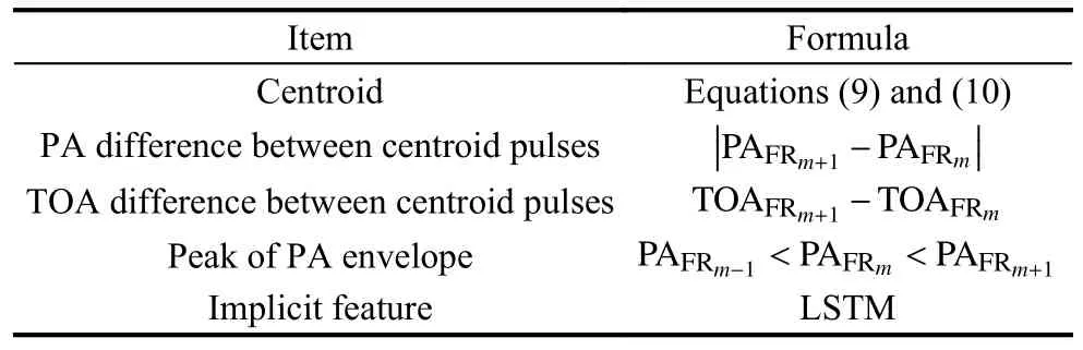
Table 1 Trajectory features

Fig.5 Schematic diagram of pulse sequence trajectory features

3.3 Separation of tracking pulses and search pulses

Consider that the trajectory variation patterns of the search pulse and the tracking pulse are different.Even if there is the influence of jitter, noise, and other situations,the trajectory change law of the search pulse can be approximated by Sinc function, and the trajectory change of the tracking pulse is approximated by linear function.Therefore, the extraction of pulses with linear variation characteristics in the pulse sequence can achieve the extraction of tracking pulses, thus completing the separation of search pulses and tracking pulses.

The reason is that the amplitude of the tracking pulse is usually larger than that of the search pulse.Peak extraction can initially filter out some of the search pulses and retain almost all of the tracking pulses and a small number of search pulses, thus improving the accuracy of detection.The specific steps of the algorithm are as follows.

The presence of tracking pulses is then determined by the double thresholds δPAFR1and δPAFR2and the number of pulses threshold δnum.

As shown in Fig.6, the red dashed lines are PAfeature1and PAfeature2.

Fig.6 HT detect

Step 3 Tracking pulse extraction.The tracking pulse extraction is based on the autocorrelation function of the peak pulse sequence itself.The PRI transform algorithm[23], which has a strong ability to suppress harmonic interference, is used to solve the variation pattern between peak pulses in the TOA dimension, i.e., PRI.Its core idea is to transform the difference in TOA (DTOA)of the pulse sequence to the spectrum.The PRI value of the pulse sequence is estimated from the position of the spectral peaks.The details are as follows.

First, the mathematical model is constructed,Tm(m=0,1,···,M-1)is the TOA of the peak pulse,whereMis the total number of pulses.And the mathematical model can be described as

where δ(t) is the unit impulse function.An integral transformationisperformedons(t) and an exponential factor exp(2πjt/τ)isintroduced.

where τ>0.|D(τ)| forms a PRI spectrum with a peak at the true PRI value.Then, the discrete formulation of the PRI transform is obtained by substitutings(t) into (19).

wherem,u∈{0,1,···,M-1} andu>m.The role of the exponential factor is to suppress subharmonic generation.Finally, based on the PRI value at the peak, a sequence search is used to extract the tracking pulse.The sequence search process is shown in Fig.7.The first pulse of the pulse sequence is the start pulse.Pulse extraction is performed at the PRI according to the search threshold ε.When Pulse 3 is successfully extracted, it is used as a new starting pulse to continue the search.The extracted pulses are tracking pulses.If the extraction fails, as shown in Pulse 5 in Fig.7, a pulse search is performed at 2PRI according to the search threshold ε.If the extraction fails for three consecutive times, the search ends and Pulse 2 is used as the starting pulse to continue the search, until the last pulse.The final extracted peak pulse is the tracking pulse {TOAtrack,PAtrack}.The remaining pulses form the search pulse {TOAsearch,PAsearch}.Together they form the centroid pulse sequence {TOAFR,PAFR},i.e.,

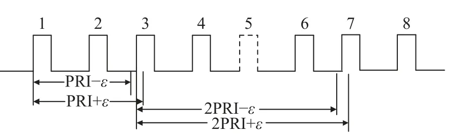
Fig.7 Sequence search schematic

3.4 Search pulses classification

3.4.1 How LSTM fits the prediction task

Deep learning technology has evolved rapidly over the past decade, and in some areas, systems based on the technology have reached or even surpassed human levels[24,25].There are two popular types of neural networks,namely, convolutional neural networks (CNNs) and RNNs [26,27].RNN is designed for processing sequential data.LSTM introduces the forgetting mechanism in the original RNN framework, which well solves the problem of gradient disappearance and successfully extracts the long-term patterns of sequence data [28-30].LSTM processes the data samples one by one in a temporal order to extract the implicit information contained in the sequence data.It can predict the upcoming data samples based on the change pattern of previous data samples.

TOA and PA features are in the form of sequence data and they contain a lot of implicit information.The law of trajectory change they present is difficult to express by traditional methods.Combining the characteristics of LSTM neural network, this section proposes to use LSTM neural network to extract the trajectory features of the pulse sequence.The pulse signal features of the next time step are predicted based on the a priori pulse signal features.In this way, we judge whether the features of the pulse signal at that moment are consistent with the trajectory change law, so as to realize the trajectory tracking of the pulse sequence and complete the search pulse classification.The LSTM neural network model is given below.

The core unit of the LSTM neural network is the memory module.Multiple identical memory modules are connected to form an LSTM neural network.The memory module contains memory cells with self-linking and gating units.The stateSt-1of the memory cell, the outputHt-1of the previous time step, and the inputXtof the current time step together determine the state vector of the internal gating cell.First, the information ofXtandHt-1is selectively filtered through the forgetting gate:

Then the information that needs to be updated is calculated.This step consists of two aspects.First, decidce which values are used to update based on the input gate:

Second, generate new candidate values based on the tanh function:

The combination of the first two steps is the process of dropping unwanted information and adding new information:

The final step is to determine the output of the model,i.e., the output gate.The information fromXtandHt-1is passed through the sigmoid function to obtain an initial outputOtas follows:

Otis multiplied pair-wise with the stateStafter the tanhactivation function to obtain the outputHtof the model:

where sigmoid and tanh are activation functions;W(·)(·)is corresponding weight matrix;B(·)is the corresponding bias; ⊙ stands for element-wise multiplication.

3.4.2 LSTM for PA envelope prediction

LSTM for PA envelope prediction is a pre-classification

If the search is successful, the corresponding pulse is extracted.If it fails, the pulse of that time step is padded by the predicted pulse and the prediction continues for the next time step.If the search fails three times in a row, the search ends, and the pulses extracted during that search are grouped into one category.Repeat the above process until the number of remaining pulses is less than three and the global search is finished.

Fig.8 Structure of LSTM for PA envelope prediction

3.4.3 LSTM for PA trajectory tracking

Envelope prediction only pre-classifies the search pulses,it also needs to track the trajectory of the pre-separated results, so as to filter out the anomalous pulses that do not conform to the trajectory change pattern of the pulse sequence.The anomalous pulse may be affiliated with the search pulse of other emitters, or it may be affiliated with the tracking pulse.In this subsection, LSTM neural network is used to extract the trajectory change pattern of pulse sequences.And the pulses of future time step are predicted according to the prior pulse sequence to determine whether the pulse of each time step conform to the trajectory change law.

Usually, the input of LSTM is equally spaced data samples, while the TOA of pulse sequences has a large randomness leading to a non-equally spaced sequence of search pulses for pre-classification.Therefore, equal interval processing of pre-classified search pulses is required before trajectory tracking.By comparing the results of segmented linear interpolation, proximity interpolation, spherical interpolation, and cubic polynomial interpolation, it is clear that cubic polynomial interpolation is optimal.Therefore, we use cubic polynomial interpolation to process the pulse sequence with equal intervals.

The structure of the trajectory tracking network based on LSTM is shown in Fig.9.First, the equally spaced processed pulse sequence is normalized and the first four PAs are used as inputs.Next, the PA predictionfor the next time step is obtained based on the processing of the LSTM layer as well as the fully connected layer.Then, the pulse at that time step is judged according to the amplitude difference threshold:

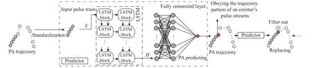
Fig.9 Structure of the trajectory tracking network based on LSTM

3.5 Tracking pulse classification

The idea of the SVC algorithm [31,32]: the data samples are transformed from the attribute space to the highdimensional feature space by a nonlinear transformation,and then the optimal hypersphere is found in this new space.This nonlinear transformation is constructed by defining a nonlinear mapping of the kernel functions.Since kernel function mapping can better distinguish,extract, and amplify useful features making them better for clustering, the tracking pulse is mapped to a highdimensional feature space by choosing a nonlinear transformationΦ.In the feature space, a closed convex hypersphere of minimum radiusRcan be found.Classification is performed based on the closed convex hyperspherical surface for tracking pulses.We omit the details of SVC here and the interested reader is referred to references[8,9].

3.6 Fusion of search pulses and tracking pulses

In tracking mode, the maximum gain of the antenna is pointed at the receiver at each moment, that is, the amplitude of each moment of the tracking pulse takes the maximum value.In the search mode, a scan cycle (corresponding to a PA envelope) in only one moment the maximum gain of the antenna pointing to the receiver, that is, a scan cycle in the search pulse in only one moment of the PA to take the maximum.Therefore, this section uses the correlation of PA between different operating modes of the same emitter to correlate and match the search and tracking pulses.Thus, the final step of homotypic radiation source signal separation is completed.

For the sake of illustration, two emitters are used here as examples.The maximum value of each envelope in the search pulse of the radiation source is first extracted and noted as

and

Then the mean values of PAsearchpeak1, PAsearchpeak2, PAtrack1,and PAtrack2are calculated separately:

4.Simulation

4.1 Simulation scene and parameter setting

4.1.1 Simulation scene

At the beginning of the study, the current experimental conditions were not able to produce realistic radiation source data.Therefore, this section uses electromagnetic environment simulation software [22] to generate homogeneous radar radiation source pulse data.And to illustrate the validity of the simulation data, a set of real pulse data is shown in Fig.10.The red and blue colors represent the tracking pulse and the search pulse, respectively.It is worth noting that real data are less available, therefore, simulation data are used to verify the effectiveness of the proposed algorithm.

Fig.10 Real pulse data

The radar emitter parameters are shown in Table 2,where the pattern of the emitter antenna is a Sinc function.A total of two scenarios are included, one for the training scenario: a reconnaissance platform versus a radar emitter platform.The pulse data in this scenario is used to train the proposed method.The other is a test scenario: one reconnaissance platform versus multiple radar platforms.The pulse data in this scenario are used to test the performance of the proposed method.And to improve the generalizability of the method, the one on one training scenario includes various forms.The motion trajectory of the reconnaissance platform and the emitter include: straight line, fold line, and curve.The motion model includes: constant velocity (CV), constant acceleration (CA), and constant turn (CT).

Table 2 Radar parameter

Experimental platform information: Intel i7 processor,4 GHz, Windows 10, 16 G memory, Matlab2018b with the deep learning toolbox.

4.1.2 LSTM model parameter setting

The LSTM network configuration parameters for PA envelope prediction are given in Table 3.Other hyperparameters: learning rate of 0.01 and number of iterations of 260.The parameters of the LSTM network for pulse sequence trajectory tracking are shown in Table 4.The learning rate is 0.004 and the number of iterations is 400.The gradient threshold for both networks is 1.If the gradient exceeds the threshold, L2 regularization is used to penalize the gradient.

Table 3 Parameter settings of LSTM for PA envelope prediction

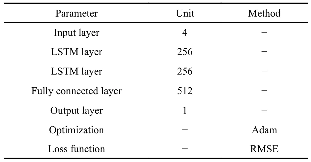
Table 4 Parameter settings of LSTM for PA trajectory tracking

4.2 Simulation results and analysis

4.2.1 Feasibility simulation verification

A typical two-plane formation is used as an example.To better simulate the real environment, pulse jitter and loss are added to the intercepted pulse sequence of the emitter for the test scenario, where jitter and loss are set to 20%respectively.The result of de-interleaving the pulse sequence is shown in Fig.11.Different colors represent different emitter.Fig.11(a) shows the real pulse distribution, and Fig.11(b) shows the de-interleaved results of the proposed method.Enlarged views of some time periods are given in Fig.11(c)-Fig.11(f).By comparing the real pulse distribution with the results in this paper, it can be seen that the overall result is satisfactory despite a small number of errors.For example, the blue envelope near 16 s in Fig.11(c).The correct result is blue, while the proposed method incorrectly classifies the peak pulse of the envelope as red.The reason for this is that the peak pulse of the search envelope is judged to be a tracking pulse when the tracking pulse is extracted, and the tracking pulse is classified as another emitter when it is classified.Then there are some errors in the two envelopes near 33 s in Fig.11(e).This is due to the LSTM network trajectory tracking prediction bias when search pulse classification is performed.The overall correct rate is 93.37%, which proves the feasibility of the proposed method.

Fig.11 Deinterleaving results

4.2.2 Comparison with other methods

In order to verify the advantages of the proposed method,a comparative experimental analysis is required.However, the premise assumptions in this paper are quite different from traditional de-interleaving methods.It is clear from the previous analysis that traditional clustering algorithms and PRI-based algorithms cannot handle the problem in this paper.To the best of our knowledge, [20] is the only paper that performs pulse de-interleaving of homogeneous radar emitters.Therefore [20] can be used as a comparison method.In addition, since the idea of the proposed method is to extract the variation pattern of pulse sequences, it can be compared with similar algorithms, including deep neural networks (DNNs) and support vector regression (SVR).

The parameters of DNN are set as follows.The number of units in the input and output layers is the same as that of LSTM neural network, and the number of units in t he hidden layer is 256 and 128.For SVR, the particle swarm optimization (PSO) algorithm is used to optimize the penalty factorCand the width parametergof the kernel function, where the range ofCis [0.1,10] and the range ofgis [0.1,20].The de-interleaving results of the four methods are shown in Table 5.

Table 5 Statistical results

The accuracy is improved by 13.28% compared to[20].The reason is that the method of [20] is equivalent to the PA envelope prediction part of the proposed method.It only considers the correlation between each envelope and does not consider the implied trajectory features of the pulses within the envelope.When the pulses are heavily overlapped, it separates many pulses that do not conform to the PA change pattern.Therefore, the correct rate of [20] is low.Compared with DNN and SVR,the correct rate is improved by 9.12% and 8.92%, respectively.Since DNN and SVR are less sensitive to sequential data than LSTM, the prediction bias of both models is larger than that of LSTM.In summary, compared with these three methods, the proposed method in this paper has better performance and proves the advantages of the proposed method.

4.3 Robust simulation

In a real combat environment, the EW receiver usually intercepts a continuous pulse sequence with many defects.For example, the arrival time uncertainty (or jitter) caused by the clock defect in the receiver timing circuit, the pulse missing caused by the pulse lower than the receiver’s sensitivity, and finally the noise in the environment.Therefore, in order to verify the robustness of the proposed method in the actual environment, noise, missing, and jitter PRI are added to the simulation data.The settings of different proportions of missing, jitter PRI,and noise and the corresponding correct rates are shown in Table 6.The pulse distribution of one set of data (missing: 20%, jitter PRI 20%, noise 10%) is shown in Fig.12.Fig.12(a) shows a set of pulse distributions.Fig.12(b)shows a 10-15 s local zoom of this set of pulses.

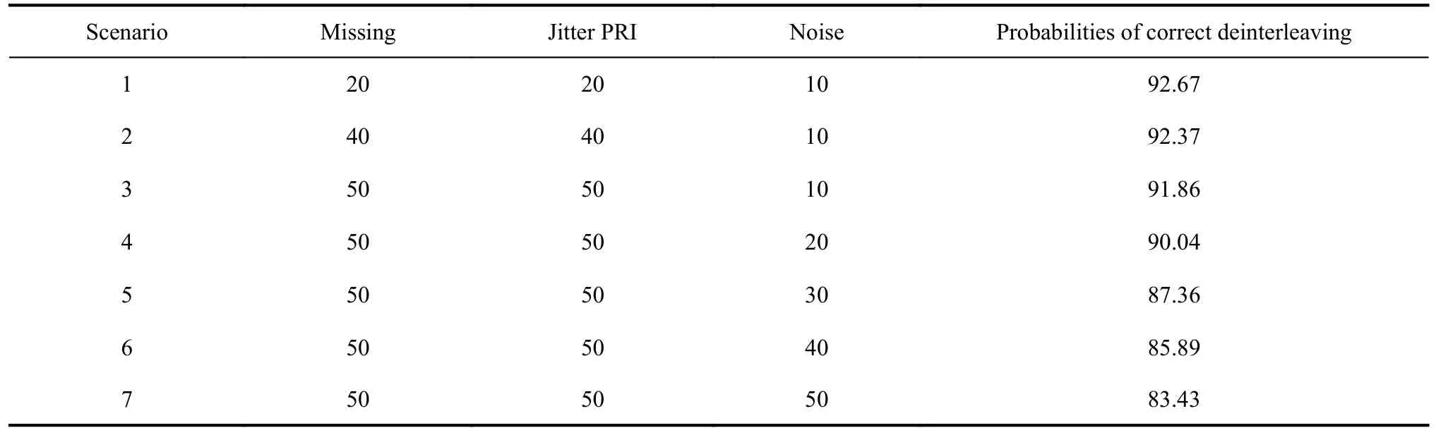
Table 6 Deinterleaving performance under different missing, jitter and noise ratios %

Fig.12 Pulse distribution with jitter (20%), missing (20%), and noise (10%)

From Table 6, it can be concluded that the loss and jitter have little impact on the performance of the proposed method, and the correct rates are above 90%.The reason is that pulse jitter and loss are specific to individual pulses, while the proposed method takes a pulse cluster(containing thousands or even tens of thousands of pulses) as a unit and extracts the centroid pulse of the pulse cluster.This way of thinking eliminates to some extent the effect of jitter and loss on the pulse variation pattern.Therefore, even if there is a large percentage of jitter and loss, it does not affect the performance of the proposed method too much.

As the percentage of noise increases from 10% to 50%,the correctness of the proposed method decreases from 91.86% to 83.43%.The reason is that the trajectory change pattern of the pulse cluster is affected when the noise ratio increases.That is, the proportion of misclassifying noise as emitter pulse increases during preprocessing; the features become inaccurate during trajectory feature extraction; the proportion of misclassification increases during tracking pulse and search pulse separation;and noise will affect the trajectory change pattern of PA during search pulse classification.Although noise can have a large impact on the performance of the algorithm,the correct rate of the proposed method is still close to 85% when the ratio of loss, jitter and noise does not exceed 50%.In summary, the robustness of the proposed method is proved to be better.

It is worth noting that although the proposed method has satisfactory performance and robustness, it also has some limitations.(i) Since the proposed method relies on the variation pattern of PA sequences, it will fail when there are artificial disturbances or multipath effects.(ii) The radar emitter of this paper is an active electronically scanned array.It only needs to change the phase of the array element to achieve the change of beam pointing.There is also a radar for mechanical scanning radar.It rotates the antenna sector periodically to achieve beam scanning.The working principles of the two are different,so the method proposed in this paper cannot be directly applied to mechanical scanning radar.Changes need to be made to the pre-processing section.

5.Conclusions

In this paper, a de-interleaving method based on the implicit features of pulse sequences is proposed.The deinterleaving problem of the same type of multi-functional radar emitter in the heavily overlapping environment of air, time, and frequency domains is solved.The proposed method extracts the trajectory variation patterns of pulse sequences through LSTM and statistical analysis to complete the de-interlacing process.Simulation experiments show that the method has satisfactory performance and robustness.In future work, we will focus on addressing the limitations of the proposed method.