Joint Probability Analysis and Prediction of Sea Ice Conditions in Liaodong Bay

LIAO Zhenkun, DONG Sheng, TAO Shanshan, , HUA Yunfei,and JIA Ning

1) College of Engineering, Ocean University of China, Qingdao 266100,China

2) Shuifa Planning and Design Co., Ltd., Jinan 250100, China

3) National Hazards Mitigation Service, Beijing 100194, China

Abstract Sea ice conditions in Liaodong Bay of China are often described by sea ice grades, which classify annual sea ice conditions based on the annual maximum sea ice thickness (AM-SIT) and annual maximum floating ice extent (AM-FIE). The joint probability distribution of AM-SIT and AM-FIE was established on the basis of their data pairs from 1949/1950 to 2019/2020 in Liaodong Bay.The joint intensity index of the sea ice condition in the current year is calculated, and the joint classification criteria of the sea ice grades in past years are established on the basis of the joint intensity index series. A comparison of the joint criteria with the 1973 and 2022 criteria revealed that the joint criteria of the sea ice grade match well, and the joint intensity index can be used to quantify the sea ice condition over the years. A time series analysis of the sea ice grades and the joint intensity index sequences based on the joint criteria are then performed. Results show a decreasing trend of the sea ice condition from 1949/1950 to 2019/2020, a mutation in 1990/1991, and a period of approximately 91 years of the sea ice condition. In addition, the Gray-Markov model (GMM) is applied to predict the joint sea ice grade and the joint intensity index of the sea ice condition series in future years, and the error between the results and the actual sea ice condition in 2020/2021 is small.

Key words sea ice grade; ice thickness; floating ice extent; Liaodong Bay; copula

1 Introduction

The sea ice of the earth is widely distributed in the Southern Ocean, Arctic Ocean, and subpolar regions (including the Baltic Sea, Sea of Okhotsk, Bering Sea, Hudson Sea,Cook Gulf, Gulf of Finland, and Bohai Sea). Sea ice in China mainly exists in the Bohai Sea and the northern part of the Yellow Sea, especially in the northernmost Liaodong Bay of the Bohai Sea (Yuanet al., 2021). Sea ice generally begins to freeze in early winter and disappears in early spring (first-year ice); it then forms on the east coast first, followed by the west coast (Maet al., 2022). The Bohai Sea has many offshore oil platforms and offshore wind farms, and the Bohai Rim has densely populated ports and a mariculture industry. Sea ice (fast and floating ice) in winter and spring can cause substantial damage to these offshore engineering structures and has a considerable impact on shipping and fishing in the Bohai Sea. The Bohai Sea is generally divided into the following five main sea areas: Laizhou Bay, Bohai Bay, Liaodong Bay, central Bohai Sea, and Bohai Strait (Fig.1). Among these areas, Liaodong Bay is located on the northeast side of the Bohai Sea,where sea ice appears yearly and the sea ice condition is the most serious.

The sea ice condition usually includes the sea ice period, extent, thickness, distribution, and drift (Zhang, 1979).For the Bohai Sea, floating ice is initially formed from the shore’s shallow sea surface in early winter. As the temperature drops, the sea water heat gradually dissipates, the thickness of the floating ice gradually increases, and the range gradually expands to the sea. Floating ice at the shallow surface of the shore further freezes and consolidates with the shore and forms fast ice. Simultaneously, the pack ice on the deep sea surface is formed by drifting with the wind and currents. Pack and fast ice reach their maximum extent and thickness in the dead of winter (generally in early February). The temperature in early spring gradually rises, and sea ice begins to melt. The sea ice thickness decreases, the floating ice decreases and melts, and the sea ice extent continues to shrink toward the shore. Finally,the fast ice melts, and the sea ice disappears.

The sea ice period refers to the time interval between the freeze and break-up dates. The longest sea ice period in Liaodong Bay is more than 120 days, and the shortest is approximately 60 days (Yang, 2000). Satellite observations show that the total sea ice extent (SIE) in the Arctic has declined across all seasons due to ongoing climate change (Stroeveet al., 2012; Stroeve and Notz, 2018;Serreze and Meier, 2019; Yadavet al., 2020). By contrast,the total SIE in the Antarctic showed a slight but persistent increasing trend from 1979 to 2015, but this trend did not continue in 2016 – 2018 (Yanget al., 2021). For the Bohai Sea, although the SIE has significant interannual variation, the trend of rising or falling is not obvious (Suet al., 2015; Sunet al., 2022). Sea ice thickness (SIT), distribution, and drift can be measured or calculated by radar,aerial remote sensing, satellite remote sensing, coastal observation stations, icebreakers, or ice-ocean coupled numerical models (Yuanet al., 2018; Yanet al., 2019; Zhanget al., 2021; Jia and Chen, 2020). Ouyanget al.(2019)studied SIT and SIE in the Bohai Sea from 2000 to 2016 and found that the increase in air temperature around the Bohai Sea had not resulted in an apparent decreasing trend in SIT and SIE over the past 16 years. Based on a coupled ocean-sea ice model, Guoet al.(2021) studied how changes in the mean state of the atmosphere in different CO2emission scenarios may affect the sea ice condition in the Bohai Sea.

The National Ocean Bureau of China established the criteria for forecasting sea ice grades in China in 1973 (Zhanget al., 2013). In this criterion, the sea ice condition in China is divided into five ice grades based on the annual maximum floating ice extent (AM-FIE) and annual maxi- mum sea ice thickness (AM-SIT), as shown in Table 1.

The distribution of sea ice in China has markedly changed in recent years due to estuary changes, coastal engineering construction, and climate change. Therefore, adjusting the original criteria is necessary. The sea ice grade in Liaodong Bay is level 1 when the AM-FIE is less than 35 n mile, according to the original criteria. However, such a situation has never occurred because the observation data of AM-FIE existed in the Bohai Sea. In addition, continuous and accurate SIT of a large area cannot be obtained. Therefore, applying AM-SIT data to determine the sea ice grade is impractical. Different from the fast ice in the polar region, the ice in the Bohai Sea is characterized by strong fluidity and small thickness; therefore, the aforementioned data are unsuitable for conducting contact measurements on the ice surface. Only SIT observations at several stations near the shore and the data obtained by the monitoring of icebreakers once or twice a year cannot reflect the overall sea ice condition. However, obtaining the AM- FIE is easy, directly reflecting the farthest offshore distance of floating ice. Therefore, the Ministry of Natural Resources of China only selected the AM-FIE as the classification index of the new criteria of China Sea Ice Grade(2022) (Criteria 2022 for short, Table 2). The SIT is also an important reference index of sea ice conditions, which is crucial in trend analysis of sea ice conditions.

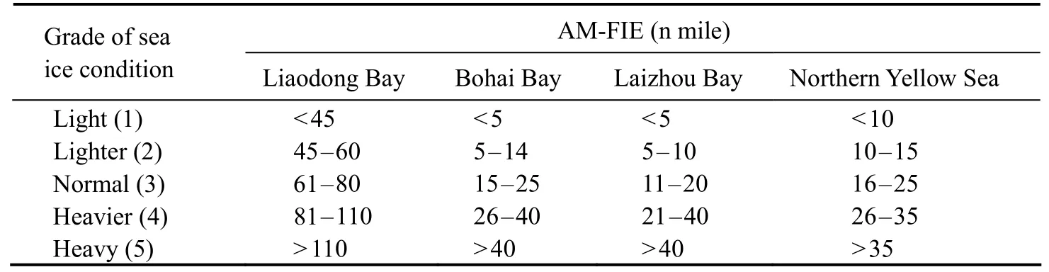
Table 2 Grades of sea ice conditions in China (2022)

In addition, different elements of sea ice conditions in a certain sea area, such as the SIT and FIE, are correlated.Therefore, studying the sea ice grade based on the correlation between the AM-SIT and AM-FIE is necessary.Donget al.(2017) investigated the joint return period oftyphoon rainfall and wind speed and defined the intensity of a typhoon according to the joint return period. The joint probability distribution of the AM-SIT and AM-FIE is constructed on the basis of the AM-SIT and AM-FIE series in Liaodong Bay using copula theory, and the joint intensity index of the sea ice condition is defined to determine a new sea ice grade criterion in Liaodong Bay. The time series analysis is then applied to estimate the trend, mutation,and period, and the Gray-Markov model (GMM) is used to predict the sea ice condition in future years.

2 Data and Methodology

2.1 Data Sources

The numerical hindcast data sequences of AM-FIE and AM-SIT in Liaodong Bay from 1949/1950 to 2019/2020 are shown in Fig.2 (denoted as 1950 – 2020 in the figure,Liuet al., 2013; Bulletin of China Marine Disaster, 1989 –2020). Herein, the SIT is the ice level thickness and refers to the vertical distance from the ice surface to the ice bottom, while the FIE refers to the distance from the bottom along the middle line of the bay to the sea ice edge (the boundary where the floating ice area meets the sea water).A new joint intensity index for the sea ice condition is proposed on the basis of marginal and joint probability analysis of the AM-FIE and AM-SIT in Liaodong Bay.

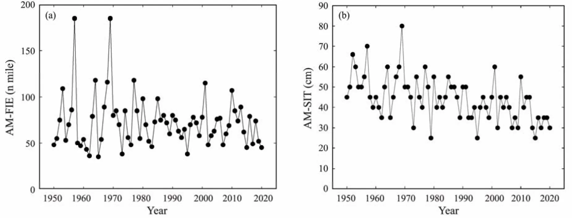
Fig.2 Series of annual maximum floating ice extent (AM-FIE) (a) and annual maximum sea ice thickness (AM-SIT) (b)in Liaodong Bay.

2.2 Marginal Probability Distributions

Suppose that the AM-FIE and AM-SIT are random variables (denoted byXandY, respectively); this study applies four kinds of univariate probability distributions (Gumbel,Weibull, lognormal, and Pearson type 3) to fit the sample of the AM-FIE or AM-SIT from 1949/1950 to 2019/2020 in Liaodong Bay.

The probability density functionsf(x) of Gumbel, threeparameter Weibull, three-parameter lognormal, and Pearson type 3 (P-III) distributions are respectively calculated as follows:

whereμ, σ, γ, μy, σy, a0,α, andβare the distribution parameters.

The parameter estimation of the four probability distributions mainly includes the moment and the maximum likelihood methods (Coles, 2007). The marginal distributions of the AM-FIE and AM-SIT should be optimized in accordance with the Kolmogorov-Smirnov (K-S) test, the average sum of squared deviationsQ, and the tail of the fitting curve (especially the upper tail).

2.3 Joint Probability Distributions

Sklar’s theorem indicates that the joint probability distribution of random variablesXandYcan be constructed on the basis of marginal distributions and by selecting an appropriate bivariate copula function. Suppose that the marginal distributions ofXandYareFX(x) andFY(y), respectively, and the optimal bivariate copula isC(u, v). The joint probability distributionFXY(x, y) of (X, Y) can then be obtained by the following formula:

This study selects three commonly used bivariate copulas, namely Clayton copula, Frank copula, and Gumbel-Hougaard (G-H) copula, to construct the joint probability distributions of the AM-FIE and AM-SIT.

The probability distributions of Clayton, Frank, and G-H copulas are respectively presented as follows:

whereθis the parameter of copula probability distributions.

The maximum likelihood method is used in this paper to estimate the marginal and joint probability distributions,and the K-S test is used to determine whether the parameter estimation of univariate curves and copula functions meets the requirements. The choice of the optimal joint probability model is substantially based on the Akaike information criterion (AIC).

The K-S test is a highly robust goodness of fit test method to determine whether the measured samples follow the selected model. The statistic of the K-S test is as follows:

The AIC value can be defined by

wherenis the sample size,kis the number of correlation parameters in the copula model, andMSEis the mean sum of squares of deviations between the empirical probability and the fitting probability, which can be defined by

A small AIC value indicates a superior fitting effect of the joint probability distribution.

2.4 Joint Intensity of Sea Ice Conditions

The joint intensity index of a bivariate annual eventE= (x, y) can be described byJI∩, which is defined as

whereXandYare the random variables of the AM-FIE and AM-SIT, respectively;xandydenote the values ofXandYin a given year, respectively;FX(x) andFY(y) are the marginal distributions ofXandY, respectively;FXY(x, y)is the joint probability distribution of (X, Y). Φ?1(?) is the inverse function of the standard normal probability distribution.

The joint intensity indexJI∩can reflect the comprehensive contribution of the FIE and SIT to the sea ice condition. TheJI∩values are used in the current study to classify the sea ice grades in Liaodong Bay. Therefore, the sample number roughly conforms to the normal distribution.

3 Results and Discussion

3.1 Optimization of Probability Distributions

The AM-FIE and AM-SIT data of Liaodong Bay are from 1949/1950 to 2019/2020 (Fig.2). Suppose that AM-FIE or AM-SIT are random variables, and the marginal and joint probability analysis is conducted to optimize the best probability model.

First, the Gumbel, Weibull, lognormal, and P-III distributions are used to fit the sequences of AM-FIE and AMSIT in Liaodong Bay. The fitting results are shown in Table 3 and Figs.3(a) and 3(b).

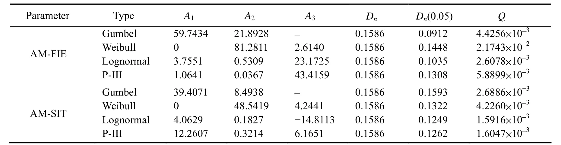
Table 3 Parameter estimation and fitting results of marginal distributions

The results shown in Table 3 indicate that under the condition of a confidence level of 0.05, the four distributions of the AM-FIE series all pass the K-S test. The table reveals that the Gumbel distribution has the smallest K-S statisticDnvalue, followed by the lognormal, P-III, and Weibull distributions. The calculated average sum of squared deviationsQvalues indicates that the lognormal distribution has the smallestQ, followed by the Gumbel, PIII, and Weibull distributions. Analysis of the overall and tail fitting of Fig.3(a) concluded that the lognormal distribution fitting is the best for the AM-FIE.

Fig.3 Fitting plots of AM-FIE and AM-SIT in Liaodong Bay. (a), AM-FIE; (b), AM-SIT.

Fig.4 Joint probability contours of AM-FIE and AM-SIT in Liaodong Bay. (a), joint probability density contours; (b), joint probability distribution contours.

Similarly, under the condition of a confidence level of 0.05, the four distributions of the AM-SIT series all passedthe K-S test. Table 3 shows that the lognormal distribution has the smallest K-S statisticDnvalue, followed by the P-III, Weibull, and Gumbel distributions. The calculated average sum of squared deviationQvalues reveals that the lognormal distribution has the smallestQ, followed by the P-III, Gumbel, and Weibull distributions.Analysis results of the overall and tail fitting of Fig.3(b)concluded that the lognormal distribution fitting is the best for the AM-SIT.

Four joint probability distributions of the AM-FIE and AM-SIT are then obtained on the basis of bivariate Clayton, Frank, and G-H copulas. The estimation of correlated parameters and model fitting tests are shown in Table 4.

Table 4 Estimation of correlated parameters and model fitting tests

The following results are observed. 1) The estimated value of ?θcorresponding to the correlated parameter of each model is within the corresponding value range. 2) The statistics of the three models all pass the K-S tests. 3) These models are in descending order according to the AIC values: G-H, Frank, and Clayton models. Therefore, the G-H model is finally selected as the joint probability distribution of AM-FIE and AM-SIT in Liaodong Bay.

The joint probability density and distribution contours of AM-FIE and AM-SIT in Liaodong Bay according to the G-H model are shown in Figs.4(a) and 4(b), respectively.

The joint intensity index of the sea ice condition in Liaodong Bay based on the AM-FIE and AM-SIT (from 1949/1950 to 2019/2020) is solved using Eq. (12), as shown in Fig.5.

Fig.5 Joint intensity index of sea ice conditions in Liaodong Bay.

3.2 New Criteria for Sea Ice Grade

New joint criteria for the sea ice grade in Liaodong Bay can be introduced on the basis of the joint intensity index values of the sea ice condition in Liaodong Bay according to the AM-FIE and AM-SIT (from 1949/1950 to 2019/2020).

The classification of sea ice grade by using the joint intensity index is based on the following principles. 1) The sea ice grades are divided into 1 to 5 with an interval of 0.5.2) The years with different sea ice grades follow an approximately normal distribution; that is, the number of years with sea ice grade 3 is the largest, followed by the number of years with sea ice grade 2.5 or 3.5, and so forth.

The new joint criteria and the classification result of the sea ice grade in Liaodong Bay are shown in Table 5, and the statistical graph is presented in Fig.6.

Table 5 New joint criteria for sea ice grade in Liaodong Bay

Fig.6 Normal distribution fitting of the years with different sea ice grades.

Three kinds of sea ice grades in Liaodong Bay can be obtained on the basis of the 1973 criteria (Table 1), 2022 criteria (Table 2), and the new joint criteria in this section of sea ice conditions (Table 5), respectively. These sea ice grade sequences from 1949/1950 to 2019/2020 are compared and plotted in Fig.7 for comparison.

Fig.7 Sea ice grade sequences obtained from the Criteria 1973, Criteria 2022, and new joint criteria.

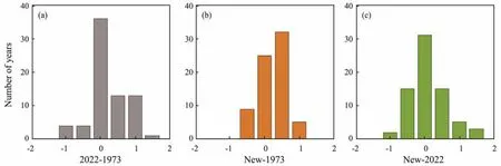
Fig.8 Differences between the grades given by different criteria.

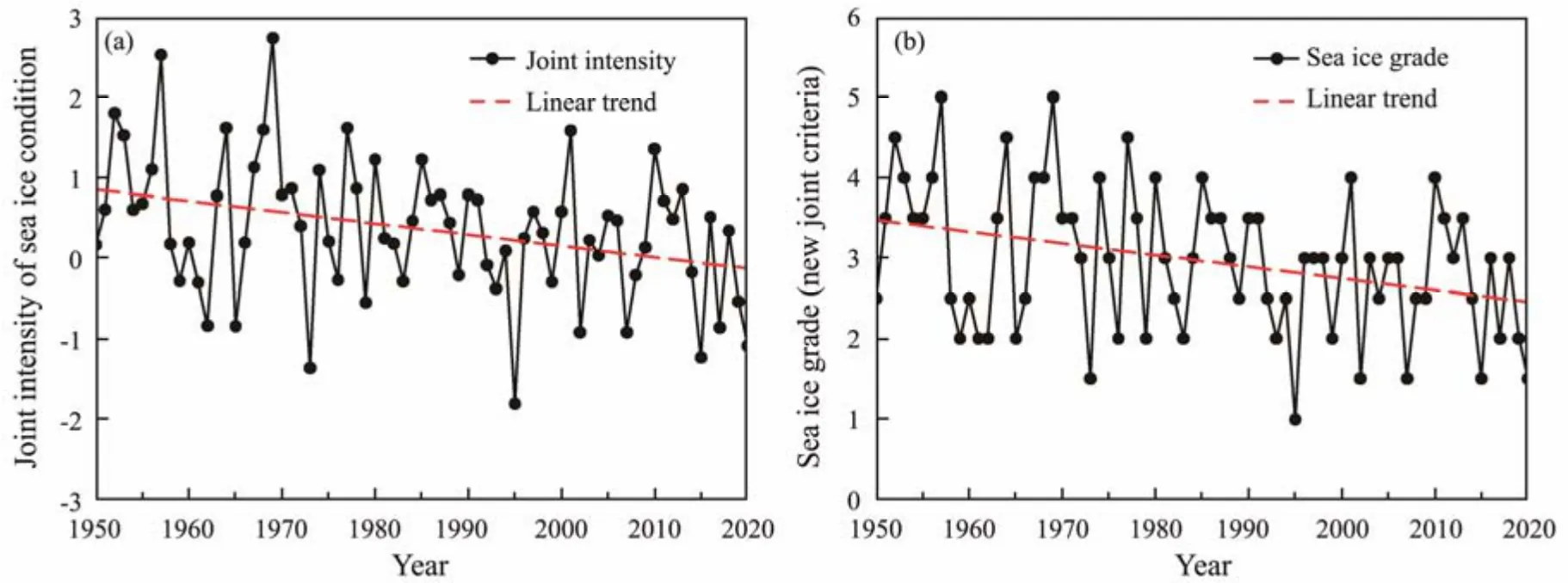
Fig.9 Joint intensity index and sea ice grade in Liaodong Bay. (a), joint intensity index of sea ice conditions; (b), sea ice grade (new joint criteria).

Fig.10 Periodograms of the joint intensity index and sea ice grade. (a), joint intensity index of the sea ice condition; (b), sea ice grade (new joint criteria).

The distributions of the differences in sea ice grade values obtained from Criteria 1973, 2022, and new joint criteria are shown in Figs.8(a), 8(b), and 8(c), respectively.

Criteria 2022 determined 27 sea ice grade values that are larger than those given by Criteria 1973. Similarly, the new joint criteria determined 41 sea ice grade values that are larger than those provided by Criteria 1973. The new joint criteria identified 23 sea ice grade values larger than those given by Criteria 2022.

Comparative results of Criteria 2022 and 1973 revealed 18 years with a difference of sea ice grade equal to or larger than 1, 36 years with the same sea ice grade, and 17 years with a difference of sea ice grade equal to 0.5. Similarly, a comparison of the new joint criteria with Criteria 1973 demonstrated only 9 years with a difference of sea ice grade equal to or larger than 1, 25 years with the same sea ice grade, and 37 years with a difference of sea ice grade equal to 0.5. Comparing new joint criteria with Criteria 2022, the difference in sea ice grade equal to or larger than 1 is only 10 years, the same sea ice grade is 31 years, and the difference in sea ice grade equal to 0.5 is 30 years. Therefore, a significant difference is observed between the sea ice grade obtained by Criteria 2022 and 1973,while the difference between the new joint criteria and Criteria 1973 or 2022 standard is insignificant. In addition,the sum of the squares of mean deviations of sea ice grade sequences obtained the following from different criteria:the difference between the new joint criteria and Criteria 1973 or 2022 (0.5070 and 0.5471, respectively) is less than that between Criteria 1973 and 2022 (0.5753).

The above discussion revealed that the new criteria of the sea ice grade given by the joint intensity index based on the AM-FIE and AM-SIT can reflect the sea ice conditions in Liaodong Bay. In sections 3.3 and 3.4, the joint intensity series of sea ice conditions (Fig.5) and the sea ice grade series are obtained by the new joint criteria (Fig.7); time series analysis and GMM are applied to access their trend, change points and period and predict the sea ice condition in future years.

3.3 Trend, Mutation, and Period

Time sequences of the joint intensity index of sea ice condition and sea ice grade based on the new joint criteria are shown in Figs.9(a) and 9(b). These sequences demonstrate a certain downward trend. Time series analysis is then used to analyze the trend, period, mutation, or jump of the sea ice condition index in Liaodong Bay.

1) Trend

Mann-Kendall trend test (Fenget al., 2020) was used to analyze the trend components of the above sequences.The results are shown in Table 6.

Table 6 Results of Mann-Kendall trend test

The trend test results show that the Mann-Kendall statistics |Z| of the sea ice grade (new joint criteria) and the joint intensity of sea ice condition are larger than the critical valueZ1?α/2(α= 0.05), and the statisticsZare less than zero. Therefore, a significant downward trend component is observed in the sequences.

2) Change point

The Pettitt change point test (Praveenet al., 2020) was used to analyze the change points of the above sequences.The results are shown in Table 7.

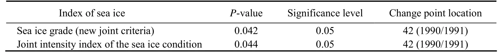
Table 7 Results of the Pettitt test

The results show that the P-values of the sea ice grade(new joint criteria) and the joint intensity index of the sea ice condition are less than the significance level of 0.05.Therefore, a significant change point component is observed in the sequence (1990/1991).

3) Period

The periodogram analyzed the periodic components of the sequences based on discrete Fourier transform (Daset al., 2021). The periodic diagrams are shown in Figs.10(a) and 10(b).

The periodic diagrams show which frequency harmonic components are included in a given sequence, and hypothesis testing identifies the significant periodic components. The results are shown in Table 8. TheFjstatistic is used in this table to test the significance of thej-th harmonics. The critical valueFαis obtained from the critical value table according to the given significance level = 0.05.Thej-th harmonic and its corresponding period are both significant whenFj>Fα. Otherwise, the corresponding period is insignificant.

Table 8 Significance test results of periodic components

The results show that the sea ice grade (new joint criteria) and the joint intensity index of the sea ice condition both have the same main harmonic frequencyωNJC=ωJI=0.069, and the corresponding period isTNJC=TJI= 91.061(year).

3.4 Prediction of Sea Ice Conditions

The GMM combines the Gray system (Deng, 1989; Liu and Lin, 2010) and the Markov chain theories. The GMM uses the traditional Gray system model GM(1, 1) to predict the trend and applied the Markov chain to forecast fluctuation values, then adds the information from the two predictions together to obtain the final prediction value (Donget al., 2012; Yeet al., 2018). GMM is applied in this study to predict the sea ice condition in Liaodong Bay in future years.

1) Sea ice grade (new joint criteria)

A series of sea ice grades (New joint criteria) from 1949/1950 to 2018/2019 is applied on the basis of the GMM to predict the sea ice grade in 2019/2020. Fig.11(a) shows the prediction curve (red line) of the sea ice grade based on GM(1, 1). Fig.11(b) reveals the prediction curve (red line)of the sea ice grade based on GMM. The model accuracy of the GMM can achieve an acceptable level. The prediction of the sea ice grade in 2019/2020 by GMM is 1.485,which is remarkably close to the actual sea ice grade of 1.5.

Fig.11 Prediction of sea ice grade in 2019/2020 based on Gray system model (GM(1, 1)) (a) and Gray-Markov model(GMM) (b).

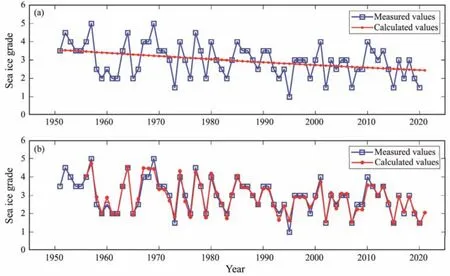
Fig.12 Prediction of sea ice grade in 2020/2021 based on GM(1, 1) (a) and GMM (b).

The sea ice grades from 1950/1951 to 2019/2020 are modeled on the basis of the GMM to predict the sea ice grade in 2020/2021. Figs.12(a) and (b) show the prediction curves (red lines) of the sea ice grade based on GM(1,1) and GMM, respectively. The model accuracy of the GMM can achieve a good level. The prediction of sea ice grade in 2020/2021 by GMM is 2.054. The AM-FIE and AM-SIE in 2020/2021 are 60 n miles and 30 cm, respectively. Therefore, its joint intensity index of sea ice condition is ?0.2665, and the corresponding sea ice grade based on Table 7 is 2.0. The prediction of sea ice grade in 2020/2021 is slightly large.

2) Joint intensity of sea ice conditions

The joint intensity series of sea ice conditions from 1949/1950 to 2018/2019 is applied to predict the joint intensity of sea ice conditions in 2019/2020 based on the GMM. Figs.13(a) and (b) show the prediction curves (red lines) of the joint intensity index of sea ice conditions based on GM(1, 1) and GMM, respectively. The model accuracy of the GMM can achieve an acceptable level.The prediction of the joint intensity value in 2019/2020 by GMM is ?1.080, which is remarkably close to the actual joint intensity value ?1.09.

The joint intensity series of sea ice conditions from 1950/1951 to 2019/2020 is modeled on the basis of GMM to predict the joint intensity series of sea ice conditions in 2020/2021. Figs.14(a) and 14(b) show the prediction curves (red lines) of the sea ice grade based on GM(1, 1) and GMM,respectively. The model accuracy of the GMM can achieve an acceptable level. The prediction of the joint intensity of sea ice conditions in 2020/2021 by GMM is ?0.495. The AM-FIE and AM-SIE in 2020/2021 are 60 and 30 cm, respectively; therefore, their joint intensity under sea ice conditions is ?0.27. The prediction of the joint intensity of sea ice conditions in 2020/2021 is slightly accurate.

4 Conclusions

In the assessment of the sea ice condition, instead of comprehensively considering the sea ice thickness and floating ice extent as independent parameters to construct the sea ice grade criteria, this paper established the joint probability distribution based on the AM-SIT and AMFIE. The joint intensity index of sea ice condition each year was calculated on the basis of the exceedance probability of the AM-SIT and AM-FIE in Liaodong Bay each year,and the joint classification criteria of the annual sea ice grade were established in accordance with the joint intensity index series.

1) The new joint criteria of the sea ice grade are effectively matched in trend with Criteria 1973 and 2022 established by the National Ocean Bureau of China, reflecting the actual sea ice condition in Liaodong Bay.

2) The joint intensity index of the sea ice condition can quantitatively reflect the annual sea ice condition in Liaodong Bay, which is more detailed than the sea ice grades.

3) The time series analysis of the series considering the joint sea ice grade and the joint intensity index revealed that the ice condition in Liaodong Bay has a downward trend, a mutation in 1990/1991, and a period of approximately 91 years of the sea ice condition.

4) A series of joint sea ice grades and joint intensity indices were modeled on the basis of the GMM, and the sea ice condition of 2020/2021 in Liaodong Bay was predicted on the basis of this model. The results show the good trend prediction capability by the GMM, and the difference between the predicted results and the actual sea ice condition has been small in the last 10 years.

Therefore, the joint probability analysis of the sea ice condition is more accurate than the previous criteria of the sea ice grades in describing the actual sea ice condition in Liaodong Bay, and the joint intensity index is a superior indicator for the analysis and prediction of the sea ice condition.

Acknowledgement

The study was supported by the National Natural Science Foundation of China (No. 52171284).