Elastic reverse-time migration based on amplitude-preserving P- and S-wave separation*

Yang Jia-Jia, Luan Xi-Wu?, Fang Gang, Liu Xin-Xin, Pan Jun, and Wang Xiao-Jie

Elastic reverse-time migration based on amplitude-preserving P- and S-wave separation*

Yang Jia-Jia1,2, Luan Xi-Wu?1,2, Fang Gang1,2, Liu Xin-Xin1,2, Pan Jun1,2, and Wang Xiao-Jie1,2

Imaging the PP- and PS-wave for the elastic vector wave reverse-time migration requires separating the P- and S-waves during the wave field extrapolation. The amplitude and phase of the P- and S-waves are distorted when divergence and curl operators are used to separate the P- and S-waves. We present a P- and S-wave amplitude-preserving separation algorithm for the elastic wavefield extrapolation. First, we add the P-wave pressure and P-wave vibration velocity equation to the conventional elastic wave equation to decompose the P- and S-wave vectors. Then, we synthesize the scalar P- and S-wave from the vector P-and S-wave to obtain the scalar P- and S-wave. The amplitude-preserved separated P- and S-waves are imaged based on the vector wave reverse-time migration (RTM). This method ensures that the amplitude and phase of the separated P- and S-wave remain unchanged compared with the divergence and curl operators. In addition, after decomposition, the P-wave pressure and vibration velocity can be used to suppress the interlayer reflection noise and to correct the S-wave polarity. This improves the image quality of P- and S-wave in multicomponent seismic data and the true-amplitude elastic reverse time migration used in prestack inversion.

Vector wavefield, reverse-time migration, PP-wave and PS-wave imaging, vector modulation, amplitude-preserving imaging

Introduction

In multiwave and multicomponent seismic exploration based on elastic wave theory instead of P-waves, the theoretical assumptions are closer to the subsurface conditions and perform better in practice. Chang and McMechan (1987) first proposed the prestack reversetime depth migration to precisely image the subsurface and obtained common imaging gathers which can be the input in AVO and AVA or other prestack depth migration methods. Subsequently, the method attracted attention and was studied extensively (Chang and McMechan, 1994; Zhang and McMechan, 2011; Yan and Xie, 2012).

Generally, there are two ways to use prestack reversetime migration of multicomponent seismic data. Thefirst is a migration method based on scalar wave theory (McMechan, 1989; Sun et al., 2006; Chattopadhyay and McMechan, 2008), which directly separates the P-and S-waves from multicomponent surface data. Then reverse-time migration extrapolates the P- and S-waves using acoustic wave equations and assuming that the vertical component is the P-wave and the horizontal component is the S-wave based on low-velocity, nearsurface seismic waves that propagate perpendicularly to the surface. When the near-surface waves do not conform to this assumption, separation errors are expected. Another migration method is the elastic RTM that is based on vector wave theory (Chang and McMechan, 1994; Sun and McMechan, 2001; He and Zhang, 2006). RTM extrapolates the multicomponent data (horizontal and vertical components) in surface reverse time. The P-and S-waves are separated in the extrapolation stage and then imaged.

The RTM method is based on extrapolation using wave equations. The migration algorithms can simultaneously process multicomponent seismic data and output P- and S-wave joint imaging results. However, the P- and S-wave fields in elastic wave equations are included in the horizontal and vertical components. The migration imaging results by crosscorrelating the horizontal and vertical components do not have a clear physical meaning and they cannot be subsequently used in interpretation and inversion. Therefore, when migrating multi-component seismic data, it is necessary to separate the P- and S-wave field from the horizontal and vertical components. The P-and S-wave field separation algorithm during wave field extrapolation is important to imaging independent P-and S-waves in RTM. In isotropic media, P-wave field is rotation-free and the S-wave field is non-divergent. P-and S-wave separation can be achieved by calculating the divergence and curl of the elastic wave field (Akiand and Richards, 1980) during the wave field extrapolation (Sun, 1999). The divergence and curl operation of the elastic wave field, which involve spatial derivatives, results in 90° phase shift and amplitude distortion (Sun et al., 2001, 2004, 2011). Sun et al. (2001) applied the Hilbert transform to the separated wave field to correct for the phase shift. Using an algorithm for the wave field separation (Sun, 1999), Sun et al. (2011) proposed a method to correct the P- and S-wave amplitude ratio using the P- and S-wave velocity ratio. Li et al. (2013) presented an accurate estimation method of near-surface velocity for the complete separation of P- and S-waves, and the P- and S-wave amplitude ratio correction, in addition, he corrected the phase in the frequency domain the phase in the frequency domain. Du et al. (2015) proposed a method to correct the amplitude error by using divergence and curl operators to separate the P-and S-wave snapshots in the wavenumber domain and multiplying by -1 the imaging amplitude for phase correction when the cross-correlation imaging condition was applied. Sun et al. (2001, 2004, 2011) and Li et al. (2013) proposed separation methods for near-surface multicomponent seismic data, and showed that the precision of the separation amplitude depend on the nearsurface velocity. Du et al. (2015) separated the wave field during the wave propagation but the separation of the wave field and amplitude correction in the wavenumber domain is computationally intensive. Phase correction is difficult to perform in noncross-correlationtype imaging conditions. Wang and McMechan (2015) proposed a vector elastic wave RTM algorithm, and added P-wave pressure, P-wave vibration velocity and S-wave vibration velocity equations into the elastic wave propagation to obtain the decomposed P- and S-waves. After imaging the modulus of the P- and S-wave vectors, the P- and S-wave imaging polarity is calculated based on the relation between the P-wave vibration direction, the S-wave vibration direction, and the reflected layer. However, there is uncertainty in the polarity of the imaging results, especially, for incident angles greater than the critical angle of the reflection.

In this study, the P-wave pressure, and the P- and S-wave vibration velocity equations are added into the conventional elastic wave equation to obtain the true amplitude of the P- and S-wave decomposition. The vector P- and S-waves are then converted to scalar P- and S-waves using the P- and S-wave propagation direction to obtain the P- and S-wave amplitude, which preserving the separation. Finally, appropriate imaging conditions are applied to the separated P- and S-waves to image the PP- and PS-wave. Numerical modeling suggests that this method can achieve the true-amplitude decomposition of P- and S-wave as well as the scalarization. During elastic wave field extrapolation, the decomposed vector P- and S-wave have the same amplitude and phase with the horizontal and vertical components before decomposition. The suppression of the migration noise of internal multiples using P-wave Poynting vector after decomposition is better than the elastic Poynting vector. Moreover, the S-wave images after the S-wave polarity correction are of superior quality compared with the ones that have not undergone S-wave polarity correction.

Elastic wave equation based on vector decomposition

Traditional elastic wave equation

Under isotropic conditions, the elatic wave equations in a two-dimensional isotropic medium are (Mu and Pei, 2005)

where vxand vzare the horizontal and vertical components of the partical vibration velocity, respectively, τxx, τzz, and τxzare the three strees components of the stress, λ and μ are the Lame elastic constants, ρ is the density of the medium, x and z are the horizonal and vertical directions of the spatial coordinates, and t is the time.

Elastic wave equation of the vector decomposition

In equation (1), the P- and S-wave components are included in the vxand vzcomponents. When jointly imaging P- and S-waves we generally calculate the divergence and curl of vxand vzduring the wave field extrapolation and separation of the P- and S-waves. Subsequently, we image the P-wave and S-wave components. The separation method is based on the divergence and curl operators and the calculation of the spatial derivatives of the vxand vzcomponents, which distort the amplitude and phase of the P- and S-waves after separation. The amplitude and phase of the separated waves differ in the vxand vzcomponents (Sun et al., 2001, 2004, 2011). To decompose the P- and S-wave vector, Xiao and Leaney (2010) proposed adding the equations for P-wave pressure, P-wave horizontal vibration velocity, P-wave vertical vibration velocity, S-wave horizontal vibration velocity, and S-wave vertical vibration velocity to the conventional elastic wave equation

where τpis the P-wave pressure, vpxand vpzare horizontal and vertical components of the P-wave vibration velocity, and vsxand vszare the horizontal and vertical components of the S-wave vibration velocity. The horizontal and vertical vibration velocity of the P-wave in equation (2) are calculated based on the vector; thus, the horizontal and vertical vibration velocity of the S-wave can be calculated by subtracting the horizontal and vertical vibration velocity of the P-wave from the full-wave vibration velocity.

Convert vector P- and S-wave field to scale wave field

The true-amplitude decomposition of P- and S-waves is obtained by combining equations (1) and (2) when performing the wavefield extrapolation. From equation (2), we know that the P- and S-wave fields after decomposition are vectors containing two components. The input to the imaging needs to be scalar P- and S-waves; thus, the vector P- and S-waves must be converted to scalar waves before imaging. Converting the vector P- and S-wave field to scalar wave field is a two-step process. First, we calculate the amplitude; the amplitudes of the scalar P- and S-wave field are the moduli of the P- and S-wave vectors. The second step is to calculate the polarity. Because the P-wave polarization direction is parallel to the P-wave propagation direction, the P-wave polarity can be obtained by calculating the inner product of the vector P-wave and P-wave propagation direction. Because the S-wave polarization direction is perpendicular to the S-wave propagation direction, the S-wave polarity can be obtained by calculating the inner product of vector S-wave and the direction of the S-wave propagation direction after 90° counter clockwise rotation. The specific equations for the scalarization of the P- and S-wave vectors are

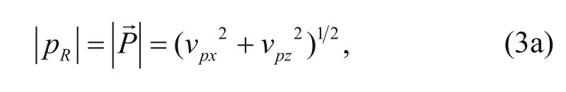
where pRand sRare the moduli of the vector P- and S-wave, respectively, andandare the Poynting vectors of the P- and S-waves, respectively. The Poynting vector is the energy flow density vector of the electromagnetic field (?erveny, 2001; Yoon and Marfurt, 2006) and shows the direction of the propagation of energy. Wang and McMechan (2015) proposed to decompose the P- and S-wave Poynting vector using the elastic wave equation

By substituting equation (4) into the equations (3b) and (3d), the polarity of the scalar P- and S-wave field can be calculated. Moreover, the positive and negativedifference between the P-wave Poynting vector of the horizontal component of the source wave field and the receiver wave field correspond to the positive or negative angle of incidence of the source wave field. Thus, we can correct the S-wave polarity, after the polarity correction, the S-wave migration results have same polarity for the positive and negative angle of incidence.

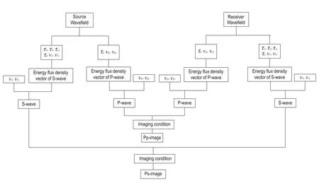
Fig.1 Flow chart of the P- and S-wave imaging in this study.

Reverse-time migration method

Figure 1 shows the flow chart for imaging the P- and S-waves. There are three steps in this process. First, we add the P-wave pressure, P-wave vibration velocity, and S-wave vibration velocity into the conventional elastic wave equation to decompose the P- and S-wave vector. Then, we use the propagation direction of the P- and S-wave and the vector P- and S-wave after decomposition to obtain the P- and S-wave field after true-amplitude separation. Next, we image the P- and S-wave field after true-amplitude separation to image the true-amplitude P- and S-wave migration.The P-wave propagation direction (Poynting vector) is calculated by using the P-wave pressure and P-wave vibration velocity, and the S-wave propagation direction (Poynting vector) is calculated by using the elastic wave field stress and S-wave vibration velocity.

Finite-differential scheme

By combining equations (1) and (2), we can decompose the P- and S-wave vector during the elastic wave field inverse time extrapolation to ensure that the amplitude and phase do not change after decomposition.

In the staggered grid space (Dong et al., 2000), by high-order difference methods to differentiate and discretize equations (1) and (2), we obtain the 2N-order difference scheme (N is random positive integer) of the elatic wave equation in a two-dimensional isotropic medium.

The specific difference scheme τxxis

where Δx and Δz are the horizontal and vertical intervals in space, respectively, Δt is the time inverval, i and j are discrete points in space, n is discrete points of time, and Ck(N)is the difference coefficient (Mu and Pei, 2005).

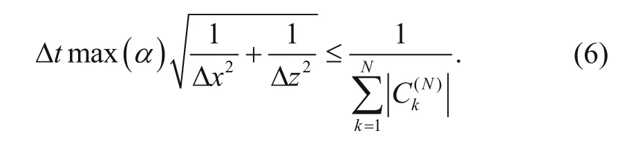
The stability condition of the above equation is the same as that of the tranditional elastic wave equation

Absorbing boundary conditions

We use the perfectly matched layer (PML) absorbing boundary conditions to solve truncation boundary problems. According to the split PML (Berenger, 1994), illustrated by the case of τxx, the absorbing boundary conditions of τxxalong the x direction is

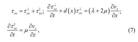
where d(x) is the damping factor along the x direction.

In the staggered grid space (Dong et al., 2000), we differentiate and discretize equation (7) using a highorder difference method to obtain the specific difference scheme of τxx

Numerical examples

Horizontal layer model

We tested the proposed algorithm by using the horizontally layered model in Figure 2. We performed forward modeling using a twelfth-order finite-difference method, a 5 m × 5 m grid, a Ricker wavelet of 30.0 Hz at (2000.0, 10.0) m, a time interval of 0.5 ms, and recording time of 2.0 s. We used the samed parameter in the reverse-time migration and the thought of the normalized wavefield separation crosscorrelation imaging based on the Poynting vector (Chen and He, 2014). We used the Poynting vector after the wavefielddecomposition and the elastic Poynting vector to suppress the interlayer reflection noise. Figure 3 shows 600 ms snapshots of the horizonal component vxand vertical component vzof the elastic wave field, the horizonal component vpxand vertical component vpzof the P-wave field, and the horizonal component vsxand vertical component vszof S-wave field. From Figure 3, we can see that the vxand vzcomponents contain information for the P- and S-waves, where as the vpxand vpzcomponents only contain information for the P-wave and the vsxand vszcomponents only contain information for the S-wave.

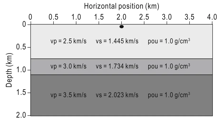
Fig.2 Horizontallayer model.

Fig.3 600 ms snapshots of each component.

To verify the amplitude preservation after the wave field decomposition, we extract the seismic traces for 1.6 km of the vxand vzcomponents, vpxand vpzcomponents, the vsxand vszcomponents, and the p and s components. The P- and S-wave components are separated owing to divergence and curl at 600 ms and the relations among the various components of the seismic trace wavelets are shown in Figure 4. Figure 4a shows the extracted seismic traces for vx, vpx, vsx, and s components at 600 ms. Figure 4b shows the extracted seismic traces for vz, vpz, vsz, and p components at 600 ms. Figure 4a also shows that the horizontal component of the P-wave (vpx) contains information for the P-wave (dispersion, noise, etc.) of the vxcomponent, the amplitude, and the phase. The information for the horizontal component of the S-wave (vsx) and the vxcomponent are in good agreement, but vsxhas high signal-to-noise ratio. This is because the vsxcomponent is extracted by subtracting the vxcomponent from the vpxcomponent. Figure 4(a2) shows that the vpxcomponent contains the noise of the vxcomponent. Aftersubtracting the noise, the vsxcomponent has high signalto-noise ratio. Moreover, the amplitude and phase in the S-wave component calculated with the curl operator do not agree with that in the vxcomponent. Similar conclusions are reached after examining Figure 4b.

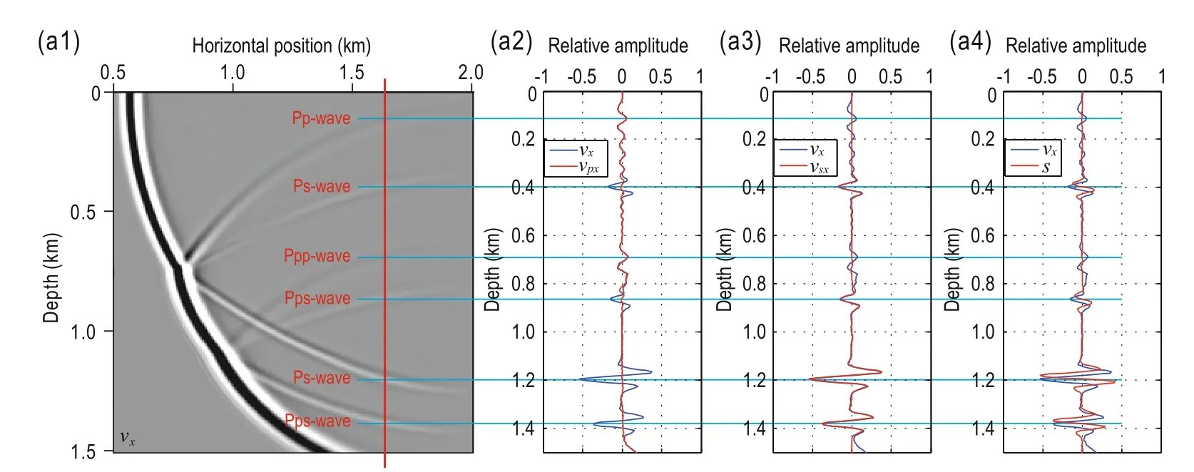
(a) Snapshots of the vxcomponent and the seismic trace of the vx, vpx, vsx, and s components in the horizontal direction at 1.6 km and t = 600 ms.

Fig.4 Seismic trace comparison between the vxand vzcomponents and P- and S-wave of each component at 1.6 km and t = 600 ms.

Figure 4 shows that using the divergence and curl operator distort the P- and S-wave amplitude and phase, which affects the imaging precision. However, using the proposed P- and S-wave decomposition preserves the amplitude. The P-wave components after decomposition are not affected by the S-wave; thus, they can be used to calculate the propagation direction of the source P-waveand this is more accurate than using the elastic wave Poynting vector.

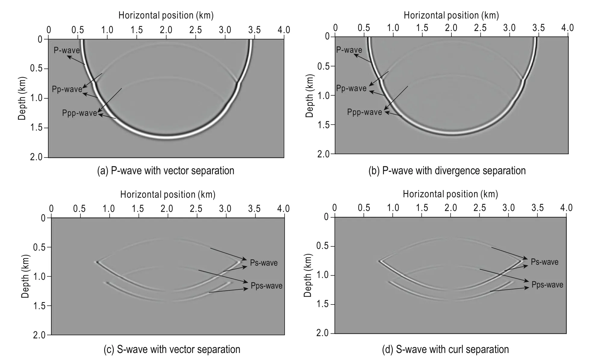
Fig.5 Snapshots comparison of the proposed vector separation algorithm and the divergence–curl separation algorithm at t = 600 ms.

Figure 5 shows forward modeling snapshots of P- and S-wave at 600 ms after separation using the proposed method and the divergence and curl operators. The separated P- and S-wave snapshots only contain information for the P- and S-wave, respectively, which implies that both methods can separate the P- and S-wave from the elastic wavefield. However, the phase of the separated P- and S-wave is different from that using the divergence and curl operators. Figure 6 shows a P-wave single-shot image using our method. Figure 6a shows aP-wave single-shot image after removing the noise using the pure P-wave Poynting vector. Figure 6b shows a P-wave single-shot image after removing the noise using the elastic wave Poynting vector. From Figure 6, we can see that the elastic wave Poynting vector does not remove the noise owing to the S-wave (red circle in Figure 6b). Because there is no S-wave energy interference in the pure P-wave Poynting vector, it is possible to remove the noise owing to the S-wave from the images and obtain P-wave images with high signal-to-noise ratio. Figure 7 shows a single-shot image of the converted S-wave using the proposed method. Figure 7a shows the converted S-wave after applying the S-wave polarity correction, whereas Figure 7b shows the converted S-wave before the polarity correction. From Figure 7, we can see that before the S-wave polarity correction, the S-wave has different polarity for positive and negative incident angle. Thus, in the migration of multi-shot data, the polarity of the S-wave can be positive or negative for the same imaging point. If not corrected, the polarity of the S-wave owing to positive and negative incident angle will superpose the positive and negative amplitude at one imaging point when stacking the S-wave imaging results, which will strongly affect the image quality of the S-wave stack. The S-wave polarity correction ensures that the stacked data have the same polarity at the same image point, enhancing the useful information and improving the signal-to-noise ratio of the migration stack sections.

Fig.6 P-wave imaging of denoising.

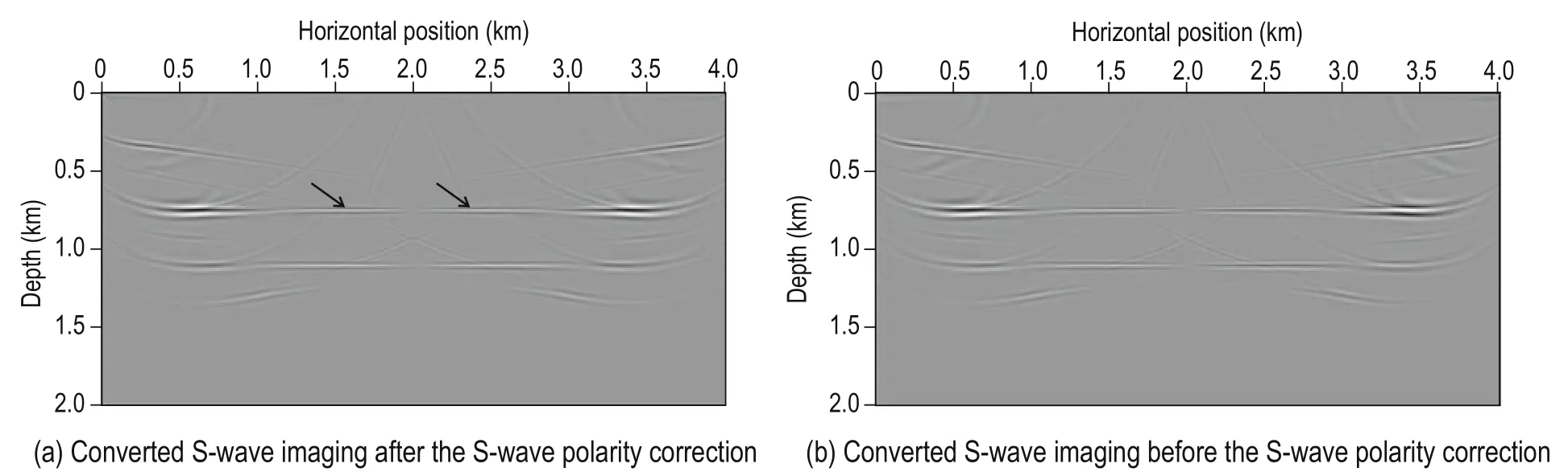
Fig.7 S-wave polarity correction comparison of converted S-wave imaging.

Marmousi elastic model

We use the Marmousi elastic wave model to test the proposed algorithm (Figure 8). The model assumes 260.0 m of seawater. The synthetic seismograms used in RTM are calculated from the first-order elastic wave equation in finite-difference forward modeling. The specific modeling parameters are the following. A Ricker wavelet 35.0 Hz at 8.0 m depth and 8.0 m intervals, 601 receivers at the sea bottom (depth 264.0 m) at 4.0 m intervals, time sampling interval of 0.1 ms, recording time of 2.5 s, and records for 301 shots. Reverse-time migration uses the same parameters as the forward modeling, moreover, we use the thought of the cross correlation of the normalized wavefield separation based on the Poynting vector (Chen and He, 2014), and use the Poynting vector after the wavefield decomposition to suppress the interlayer reflection noise.

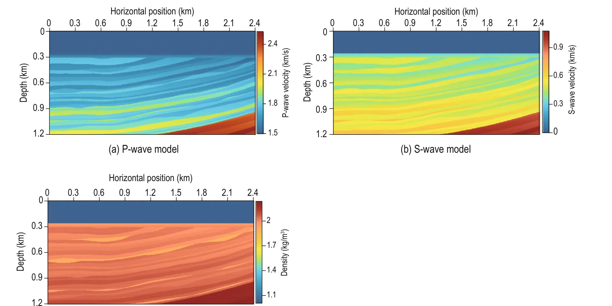
(c) Density modelFig.8 Marmousi-II elastic model.

Figure 9 shows 700 ms snapshots of the wave field forward modeling before the separation. Figure 10 shows the P- and S-wave separation snapshots using the proposed method and the divergence–curl method. Figure 9 show that vpxand vpzcomponents contain information for the P-wave, whereas the vsxand vszcomponents contain information for the S-wave. The proposed method can decompose the P- and S-waves in a complex model. Figure 10 shows that both methods separate the P- and S-waves but the proposed method has better resolution. Figure 11 shows the P-wave and converted S-wave migration stack profiles. Figure 11a shows the P-wave migration stack profile using the separated P-wave based on the proposed method and the Poynting vector of the P-wave after vector decomposition to suppress the interlayer reflection noise. Figure 11b shows the converted S-wave migration stack profile before the S-wave polarity correction using the proposed method. Figure 11c shows the converted S-wave migration stack profile after the S-wave polarity correction using the proposed method and using the P-wave vibration velocity after decomposition for S-wave polarity correction. Figure 11a shows that the structures in the P-wave migration stack profile are clear, the low-frequency noise owing to the interlayer reflection noise is better suppressed, and the imaging resolution is high. Clearly, the proposed method can image complex models. From Figure 11b, we can seethat the converted S-wave migration stack profile before the S-wave polarity correction is affected by the different shots of the same imaging point with different polarities. The imaging result is discontinuous. However, the events of the converted S-wave migration stack profile have better continuity and higher signal-to-noise ratio after the S-wave polarity correction (Figure 11c).

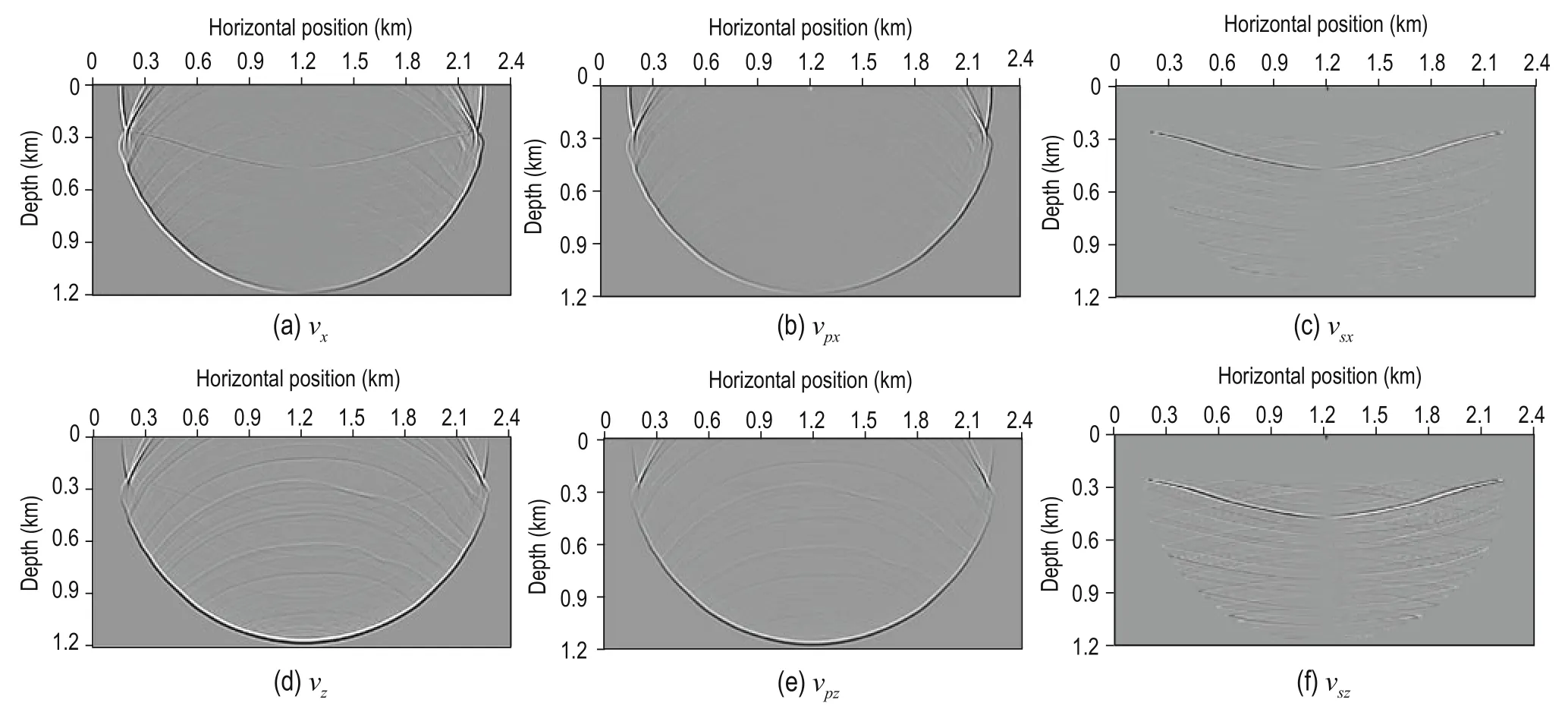
Fig.9 700 ms snapshots of each component.

Fig.10 700 ms snapshots comparison between the proposed vector separation algorithm and the divergence-curl separation algorithm.

Fig.11 Imaging of P-wave and converted S-wave after and before the S-wave polarity correction.

Conclusions

Based on the vector decoupling elastic wave equation, we present a P- and S-wave amplitude-preserving separation algorithm during elastic wave extrapolation. The algorithm adds the P-wave pressure, P-wave vibration velocity, and S-wave vibration velocity equations in the conventional equations to decompose the P- and S-wave vectors. We then use the Poynting vector of pure P- and S-wave after decomposition to convert the vector P- and S-waves to scalar wave fields.

The proposed method has the following characteristics. (1) There is a small increase in the calculation time despite the added equations. (2) The proposed wave vector algorithm can decompose the P- and S-wave vectors without amplitude and phase distortion. (3) The precision of scalarizing the P- and S-wave vectors depends on the calculation of the P- and S-wave propagation direction. We calculate the P- and S-wavepropagation direction using the pure P- and S-waves after decomposition. Uncertainties are introduced by model complexities. In the future, we will focus on how to calculate the P- and S-wave propagation direction in the elastic wave field extrapolation.

Acknowledgment

We would like to thank Dr. He Bingshou for suggestions and constructive comments.

Aki, K., and Richards, P. G., 1980, Quantitative seismology, theory and methods: W. H. Freeman and Co, San Francisco. Berenger, J. P., 1994, A perfectly matched layer for the absorption of electro-magnetic waves: Journal of Computational Physics, 114, 185-200.

?erveny, V., 2001, Seismic ray theory: Cambridge University Press, England.

Chang, W. F., and McMechan, G. A., 1987, Elastic reversetime migration: Geophysics, 52(10), 1365-1375.

Chang, W. F., and McMechan, G. A., 1994, 3D elastic prestack reverse-time depth migration: Geophysics, 59(4), 597-609.

Chattopadhyay, S., and McMechan, G. A., 2008, Imaging conditions for reverse time migration: Geophysics, 73(3), S81-S89.

Chen, T., and He, B. S., 2014, A normalized wavefield separation cross-correlation imaging condition for reverse time migration based on Poynting vector: Applied Geophysics, 11(2), 158-166.

Dong, L. G., Ma, Z. T., Cao, J. Z., et al., 2000, A staggeredgrid high-order difference method of one-order elastic wave equation: Chinese Journal of Geophysics(in Chinese), 43(3), 411-419.

Du, Q. Z., Zhang, M. Q., Chen, X. R., Gong, X. F., and Guo, C. F., 2015, True-amplitude wavefield separation using staggered-grid interpolation in the wavenumber domain: Applied Geophysics, 11(4), 437-446.

He, B. S., and Zhang. H. X., 2006, Vector prestack depth migration of multi-component wavefield: Oil Geophysical Prospecting (in Chinese), 41(4), 369-374.

Li, Z. Y., Liang, G. H., and Gu, B. L., 2013, Improved method of separating P- and S-waves using divergence and curl: Chinese Journal of Geophysics (In Chinese), 565(6), 2012-2022.

McMechan, G. A., 1989, A review of seismic acoustic imaging by reverse-time migration: International Journal of Imaging Systems and Technology, 1(1), 18-21.

Mu, Y. G., and Pei, Z. L., 2005, Seismic numerical modeling for 3-D complex media: Petroleum Industry Press, China (in Chinese).

Sun, R., 1999, Separating P- and S-waves in a prestack 2-dimensional elastic seismogram: 61st Conference, European Association of Geoscientists and Engineers, Extended Abstracts, 6-23.

Sun, R., Chow, J., and Chen, K. J., 2001, Phase correction in separating P- and S-waves in elastic data: Geophysics, 66(5), 1515-1518.

Sun, R., and McMechan, G. A., 2001, Scalar reversetime depth migration of prestack elastic seismic data: Geophysics, 66(5), 1519-1527.

Sun, R., McMechan, G. A., and Chuang, H., 2011, Amplitude balancing in separating P and S-waves in 2D and 3D elastic seismic data: Geophysics, 76(3), S103-S113.

Sun, R., McMechan, G. A., Hsian, H., and Chow, J., 2004, Separating P- and S-waves in prestack 3D elastic seismograms using divergence and curl: Geophysics, 69(1), 286-297.

Sun, R., McMechan, G. A., Lee. C. S., et al., 2006, Prestack scalar reverse-time depth migration of 3D elastic seismic data: Geophysics, 71(5), 199-207.

Wang, W. L., and McMechan, G. A., 2015, Vector-based elastic reverse time migration: Geophysics, 80(6), S245-S258.

Xiao, X., and Leaney, W. S., 2010, Local vertical seismic profiling (VSP) elastic reverse-time migration and migration resolution — Salt-flank imaging with transmitted P-to-S waves: Geophysics, 75(2), S35–S49.

Yan, R., and Xie, X., 2012, An angle-domain imaging condition for elastic reverse time migration and its application to angle gather extraction: Geophysics, 77(5), S105–S115.

Yoon, K., and Marfurt, K. J., 2006, Reverse-time migration using the Poynting vector: Exploration Geophysics, 37, 102–107.

Zhang, Q., and McMechan, G. A., 2011, Common-image gathers in the incident phase-angle domain from reverse time migration in 2D elastic VTI media: Geophysics, 76(6), S197–S206.

Yang Jia-Jia, got her PhD Degree in geophysical prospecting from Ocean University of China in 2015. Now she works in Qingdao Institute of Marine Geology as a post-doctoral. Her research interests are seismic wave theory, multi-technology and multi-component seismic wave reverse-time depth migration.

Manuscript received by the Editor April 1, 2016; revised manuscript received September 1, 2016.

*This work is supported by Special Research Grant for Non-profit Public Service (No. 201511037), National Natural Science Foundation of China (No. 41504109, 41506084, and 41406071), China Postdoctoral Science Foundation (No. 2015M582060), and Qingdao Municipal Applied Research Projects (No. 2015308).

1. Key Laboratory of Marine Hydrocarbon Resources and Environmental Geology, Ministry of Land and Resources, Qingdao Institute of Marine Geology, Qingdao 266071, China;

2. Laboratory for Marine Mineral Resources, National Laboratory for Marine Science and Technology, Qingdao 266071, China.

?Corresponding author: Luan Xi-Wu (Email: xluan@cgs.cn)

? 2016 The Editorial Department of APPLIED GEOPHYSICS. All rights reserved.