Stability Estimates of High Order Continuous Interior Multi-Penalty Finite Element Method for Helmholtz Equation with High Wave Number
2019-03-30 08:22ZHULingxue朱凌雪
應用數學 2019年2期
ZHU Lingxue(朱凌雪)
(Department of Mathematics,Jinling Institute of Technology,Nanjing 211169,China)
Abstract: Some continuous interior multi-penalty finite element method (CMP-FEM) of using piecewise polynomials of order p≥2 for the Helmholtz equation in the two and three dimensions is considered.The proposed CMP-FEM is stable (hence well-posed) for any k,h,p and penalty parameters with positive imaginary parts,where k is the wave number,h is the mesh size.
Key words: Helmholtz equation;Large wave number;Stability estimate;CMP-FEM
1.Introduction
This paper is devoted to stability estimates of some continuous interior multi-penalty finite element method (CMP-FEM) for the following Helmholtz problem:
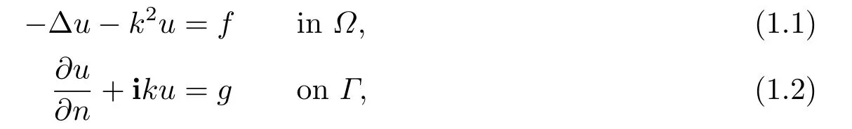
where? ?Rd,d= 2,3,is a domain with smooth boundary,Γ:=??,denotes the imaginary unit,andndenotes the unit outward normal to??.The above Helmholtz problem is an approximation of the acoustic scattering problem (with time dependence eiωt) andkis known as the wave number.The Robin boundary condition (1.2) is known as the first order approximation of the radiation condition[1].We remark that the Helmholtz problem (1.1)-(1.2)also arises in applications as a consequence of frequency domain treatment of attenuated scalar waves[2].
The CIPFEM,which was first proposed by Douglas and Dupont[3]for elliptic and parabolic problems in 1970’s and then successfully applied to convection-dominated problems as a stabilization technique[4?8],uses the same approximation space as the FEM but modifies the bilinear form of the FEM by adding a least squares term penalizing the jump of the gradient of the discrete solution at mesh interfaces.More recently,the CIPFEM has shown great potential for simulating Helmholtz scattering problems with high wave number[9?12].We remark that the idea of penalizing the jump of the gradient of the discrete solution is also used in the interior penalty Galerkin methods (IPDG)[13?18].
Our trick is used to prove the absolute stability of the CMP-FEM,which mimics the stability analysis for the PDE solutions given by[19–21]and makes use of the so-called Oswald interpolation[6,22?23].The choice of complex penalty parameters with positive imaginary parts is needed to make this trick work.We remark that the technique for deriving the stability of the linear CIP-FEM developed in[9]does not work for higher order methods because it relies on the fact of ?uh=0 on each element.
The remainder of this paper is organized as follows.In Section 2,we first introduce notation and then formulate our CMP-FEM.Section 3 is devoted to the stability analysis for the CMP-FEM proposed in Section 2.It is proved that the proposed CMP-FEM is stable(hence well-posed) without any mesh constraint.
Throughout the paper,Cis used to denote a generic positive constant which is independent ofh,p,k,f,gand the penalty parameters.We also use the shorthand notationABandBAfor the inequalityA ≤CBandB ≥CA.ABis a shorthand notation for the statementABandBA.We assume thatk ?1 since we are considering high-frequency problems.For ease of presentation,we assume thatkis constant on?.We also assume that?is a strictly star-shaped domain with an analytic boundary.Here“strictly star-shaped”means that there exist a pointx? ∈?and a positive constantc?depending only on?such that

2.Formulation of CMP-FEM
To formulate our CMP-FEM,we first introduce some notation.The standard space,norm,and inner product notation are adopted.Their definitions can be found in [24-25].In particular,(·,·)QandforΣ ??Qdenote theL2-inner product on complex-valuedL2(Q)andL2(Σ) spaces,respectively.Define (·,·) := (·,·)?andFor simplicity,Define‖·‖j:=‖·‖Hj(?)and|·|j:=|·|Hj(?).
LetThbe a curvilinear triangulation of?[26?27],which consists of elements which are the images of the reference element.For anyK ∈Th,we definehK:= diam(K).Similarly,for each edge/faceeofK ∈Th,definehe:= diam(e).Leth= maxK∈Th hK.Assume thathKh.Denote bythe reference element and byFKthe element maps fromtoK ∈Th.
LetVhbe the approximation space of piecewise mappedp-th order polynomials,that is,

wherePp() denotes the set of all polynomials whose degrees do not exceedpon.
We define
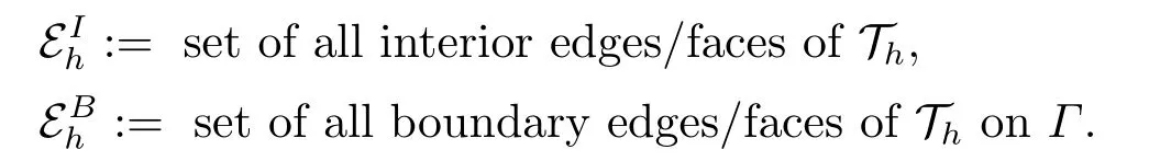
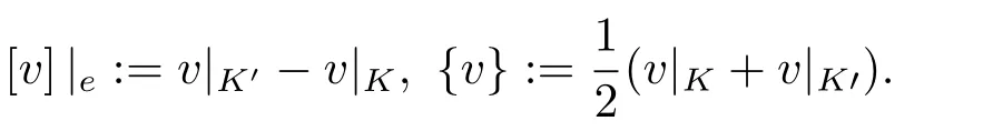
For everye=?K ∩?K′ ∈EIh,letnebe a unit normal vector toe.For everye ∈EBh,letne=nthe unit outward normal to??.We assume that the normal vectorneis oriented fromK′toKand define
Letp ≥2 be a fixed integer,which will be used to denote the degree of thehp-CMP methods in this paper.For each integer 2≤q ≤p,we define the“energy” spaceVand the sesquilinear formaqh(·,·) onV ×Vas follows:

where

andγ1,e,··· ,γq,eare nonnegative numbers.
Then our CMP-FEM is defined as follows: Finduqh ∈Vhsuch that

Remark 2.1(i) Clearly,if the parametersγj,e ≡0,j= 1,2,··· ,q,then the CMPFEM becomes the standard FEM.(ii)Penalizing the jumps of normal derivatives (i.e.,theJ1term above) was used early by Douglas and Dupont[2]for second order PDEs and by Babuˇska and Zl′amal[28]for fourth order PDEs in the context ofC0finite element methods,by Baker[29](with a different weighting,also see [30]) for fourth order PDEs.The idea of using multi-penaltiesJ0,J1,··· ,Jpwith positive penalty parameters was first used by Arnold[13]for coercive elliptic and parabolic PDEs.
The following (semi-)norm on the spaceVis useful for the subsequent analysis:

3.Stability Estimates for the CMP-FEM
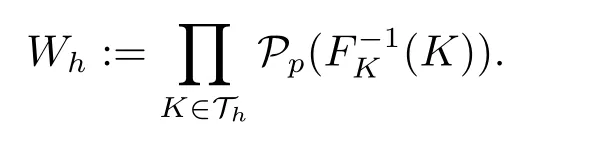
Some stability estimates have been proved for the discontinuous Galerkin methods[15?16,31]and the spectral-Galerkin methods[32].Their analyses mimic the stability analysis for the PDE solutions given in [19–21].The key idea is to use the test functionsv=uhandv=(x ?x?)·?uh,respectively,and to use the Rellich identity(for the Laplacian),wherex?is a point such that the domain?is strictly star-shaped with respect to it (see (1.3)).As for our CMP-FEM (2.3),although the test functionvh=uhcan still be used,the test functionvh=(x ?x?)·?uhdoes not apply since it is discontinuous and hence not in the test spaceVh.We get around this difficulty by taking theL2projection of (x ?x?)·?uhto the finite element spaceVh.To analyze the error of theL2projection,we recall the so-called Oswald interpolation operatorIOs,which has been analyzed in [6,22-23].LetWhbe the space of(discontinuous) piecewise mapped polynomials:
Lemma 3.1There exists an operatorIOs:Wh Vhand a constantCpdepending only onpsuch that for allK ∈Th,the following estimate holds:
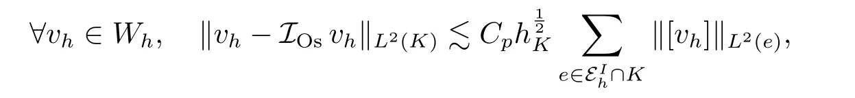
whereCp=p?1for Cartesian meshes andfor triangulations (d=2,3).
Lemma 3.2LetQhbe theL2projection ontoVhand letCpbe the constant in Lemma 3.1.Then the following estimates hold:
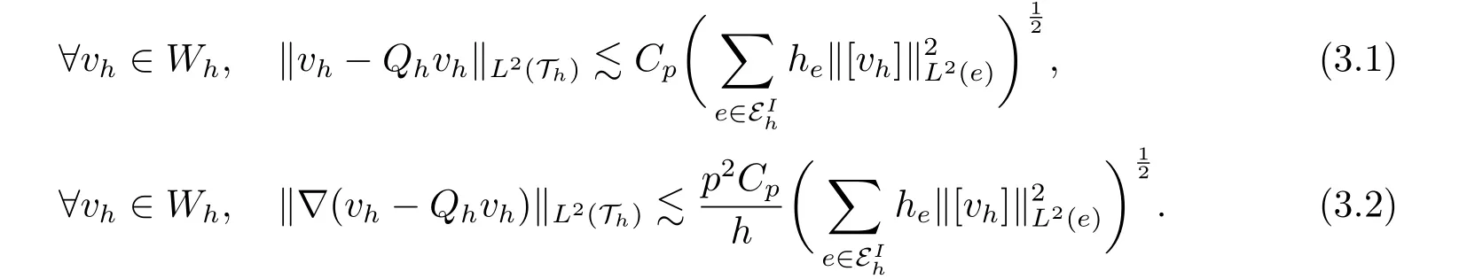
ProofThe equation (3.1) follows from‖vh ?Qhvh‖L2(Th)≤‖vh ?IOsvh‖L2(Th)and Lemma 3.1.The equation (3.2) follows from the inverse inequality and (3.1).
We cite the following lemma,which establishes two integral identities that play a crucial role in our analysis.
Lemma 3.3[15]Then there hold
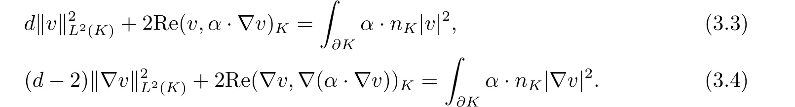
Herex?is a point such that the domain?is strictly star-shaped with respect to it(see(1.3)).
Remark 3.1The identity (3.4) can be viewed as a local version of the Rellich identity for the Laplacian ?[20].
We need the following trace and inverse inequalities[6,33].
Lemma 3.4For anyK ∈Thandz ∈Pp(F?1K(K)),

Now,takingvh=uqhin (2.3) yields

Therefore,taking the real part and the imaginary part of the above equation we get the following lemma.
Lemma 3.5Letuqh ∈Vhsolve (2.3).Then
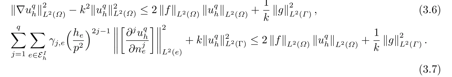
From(3.6)and(3.7)we can bound‖?uqh‖L2(?)and the jumps in terms of‖uqh‖L2(?)acrosse ∈EIh.In order to get the desired a priori estimates,we need to derive a reverse inequality whose coefficients can be controlled.Such a reverse inequality,which is often difficult to get under practical mesh constraints,and stability estimates foruqhwill be derived next.
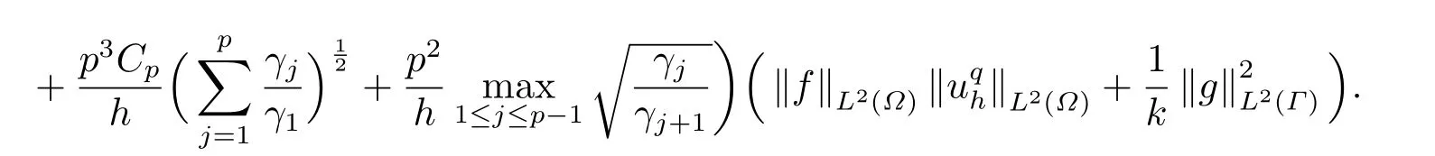
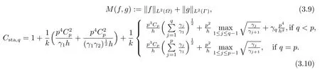
Theorem 3.1Letuqh ∈Vhsolve(2.3)and supposehK,heh,γj,e ?γj,j=1,2,··· ,q.Then

where
ProofWe divide the proof into three steps.
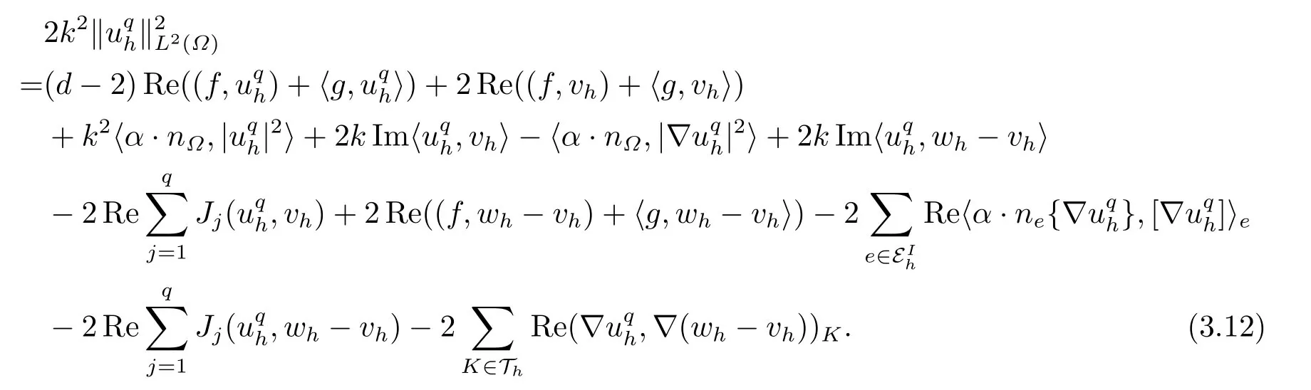
Step 1 Derivation of a representation identity for‖uqh‖L2(?).Definevhbyvh|K=α·?uqh|Kfor everyK ∈Th,denote bywh=Qhvh,and hencewh ∈Vh.Using thiswhas a test function in (2.3) and taking the real part of resulting equation we get

It follows from (3.3),(3.5) and (3.11) that
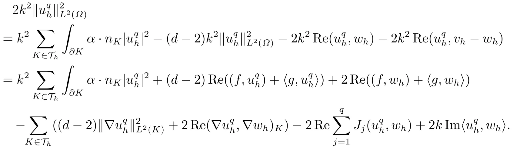
Since the terms on the right-hand side of the above equality can be mined in the exact same way as in [10],we omit their derivations and only give the final results here.
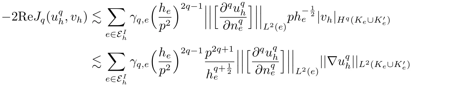
Step 2 Derivation of a reverse inequality.We bound each term on the right-hand side of the above equality.Some terms can be bounded in the exact same way as in [10],we omit their derivations and only give the final results here for the reader’s convenience.
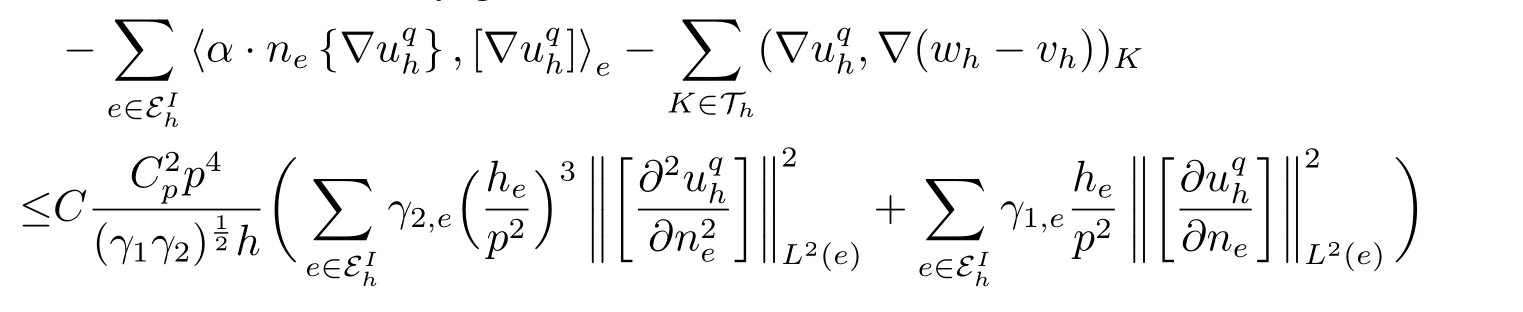

By direct calculations we get that on each edge/faceeofK ∈Th,

wheredenote an orthogonal coordinate frame on the edge/face

Here we have used the fact that (p+1)th order derivatives ofuqhare zero becauseuqhis a polynomial of degree at mostp.
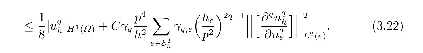
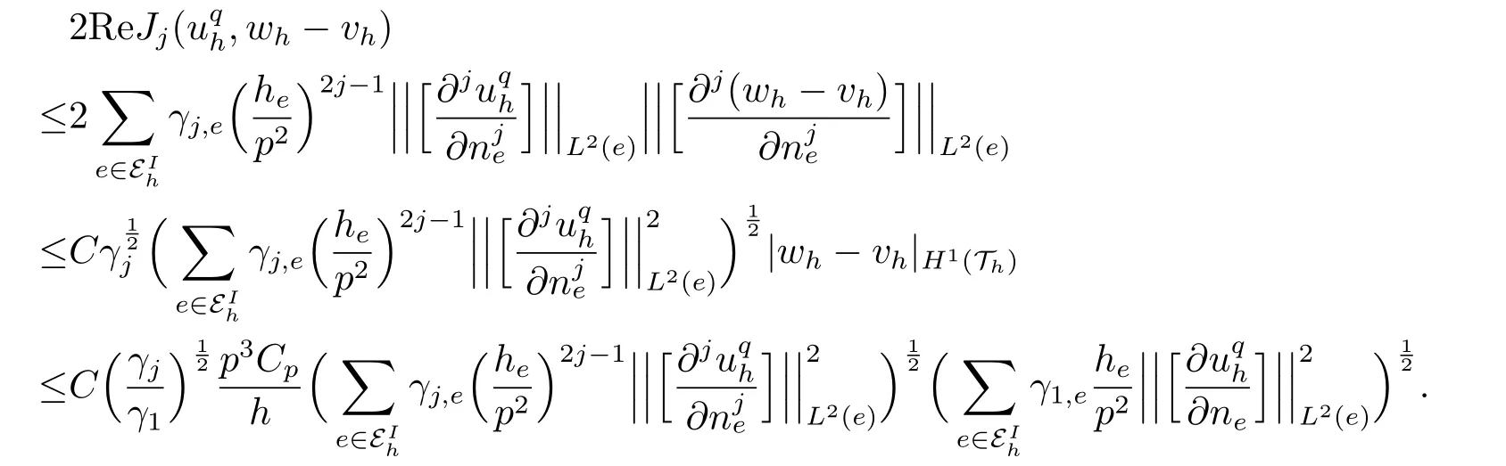
Forj=1,2,··· ,q ?1,by (3.19) and inverse inequalities (cf.Lemma 3.4) we have
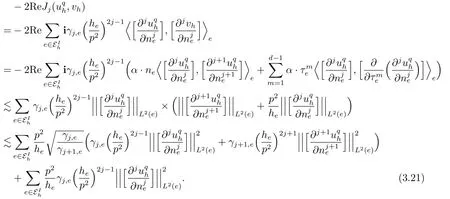
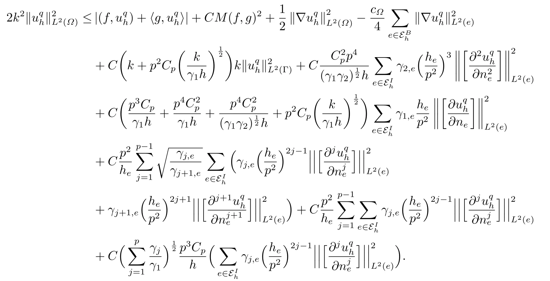
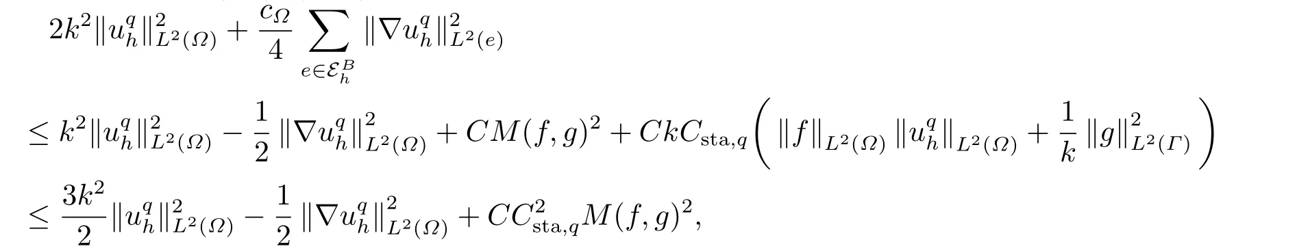
Ifq Ifq=p,(3.20) and the definition ofJp(·,·) immediately imply that Forj=1,2,··· ,q,from (5.24)[10]and Lemma 3.4, Therefore, Step 3 Finishing up.We only prove the case ofq=psince the proof forq It follows from (3.6),(3.10),and the above inequality that which together with (3.7) implies (3.8).The proof is completed. Remark 3.2Clearly,if we choosethenwhereCpis defined in Lemma 3.1.Recall that the best stability constant obtained so far for thehp-IPDG method isby Theroem 3.3 in [16]. Since the scheme (2.3) is a linear complex-valued system,an immediate consequence of the stability estimates is the following well-posedness theorem for (2.3). Theorem 3.2The CMP-FEM (2.3) has a unique solutionuqhfork >0,h >0,andγ1,··· ,γq >0.