Applying physics informed neural network for flow data assimilation ＊

Xiao-dong Bai, Yong Wang, Wei Zhang

1. Ministry of Education Key Laboratory of Coastal Disaster and Defence, Hohai University, Nanjing 210098,China

2. Max Planck Institute for Dynamics and Self-Organization, G?ttingen, Germany

3. Science and Technology on Water Jet Propulsion Laboratory, Marine and Research Institute of China,Shanghai 200011, China

Abstract: Data assimilation (DA) refers to methodologies which combine data and underlying governing equations to provide an estimation of a complex system. Physics informed neural network (PINN) provides an innovative machine learning technique for solving and discovering the physics in nature. By encoding general nonlinear partial differential equations, which govern different physical systems such as fluid flows, to the deep neural network, PINN can be used as a tool for DA. Due to its nature that neither numerical differential operation nor temporal and spatial discretization is needed, PINN is straightforward for implementation and getting more and more attention in the academia. In this paper, we apply the PINN to several flow problems and explore its potential in fluid physics. Both the mesoscopic Boltzmann equation and the macroscopic Navier-Stokes are considered as physics constraints.We first introduce a discrete Boltzmann equation informed neural network and evaluate it with a one-dimensional propagating wave and two-dimensional lid-driven cavity flow. Such laminar cavity flow is also considered as an example in an incompressible Navier-Stokes equation informed neural network. With parameterized Navier-Stokes, two turbulent flows, one within a C-shape duct and one passing a bump, are studied and accompanying pressure field is obtained. Those examples end with a flow passing through a porous media. Applications in this paper show that PINN provides a new way for intelligent flow inference and identification,ranging from mesoscopic scale to macroscopic scale, and from laminar flow to turbulent flow.

Key words: Data assimilation (DA), deep learning, physics informed neural network, hydrodynamics

Introduction

Data assimilation (DA), integrating data (normally obtained by measurements) for numerical studies,becomes more and more important in areas of atmosphere and ocean, as it benefits from both the data and the modelling[1]. It has also been introduced into fluid mechanics[2-3]. Meanwhile, machine learning is now a powerful technique for studying fluid mechanics partially due to the proliferation of largescale computing capability. With proper informationprocessing algorithms, machine learning can be used in flow modeling, flow control and optimization.Based on the labeled data used in training, machine learning can be generally categorized into three types:the supervised, semi-supervised and unsupervised machine learnings. The supervised machine learning provides a mapping function between labeled input and output data, while the unsupervised one clusters unlabeled dataset and provides the hidden mechanism of a specific phenomenon. The semi-supervised machine learning is a hybrid type that employs labeled and unlabeled data for training. For example, deep rein-forcement learning, as a semi-supervised strategy,has been successfully applied in hydrodynamics of fish-stock flow control, drag reduction, etc.[4]. The widely used dynamic mode decomposition method[5-7]in fluid physics is basically an unsupervised machine learning. An extensive review on machine learning for fluid mechanics can be found in Brunton et al.[8].

In the area of fluid modeling, machine learning has gained considerable progress. Tracey et al.[9]used a modified kernel regression supervised learning method to model the anisotropy part of Reynolds stress of turbulence. Later on, the authors[10]tried a single-layer neural network to reconstruct the source term of the Spalart-Allmaras turbulence model. Similarly, Zhang et al.[11]used the DNS data to train a tensor based deep neural network (DNN). Using the DNS data of turbulent flows, Ling et al.[12]trained a deep learning neural network incorporating the Galilean invariance and established mathematical model of Reynolds stress. Numerical results showed that the trained model can improve the turbulent flow prediction over wavy plates. Weatheritt and Sanderberg[13]developed a multi-dimensional gene expression programming (MGEP) algorithm and introduced an additional algebra term in order to reduce discrepancy and calibrate closure coefficients of the quadratic eddy-viscosity models. Zhang et al.[14]developed a data-driven, physics-informed Bayesian framework for quantifying and reducing uncertainties in Reynolds-averaged Navier-Stokes (RANS)simulations. Their simulation delivered better quantities though with sparse observations.

Despite achievements in flow modeling, machine learning method is more extensively explored for challenging flow problems, instead of serving as a“black-box”, as pointed out by Brunton et al.[8]Recently, Raissi et al.[15]proposed a physics informed neural network (PINN) to solve and discover physics involving complex partial differential equations (PDE),such as the nonlinear advection-diffusion equation, the Korteweg-de Vries (KdV) equations and the Schr?dinger equation. It is demonstrated that the PINN has an encouraging ability to solve complex physics phenomena, including shock, bifurcation, etc.In a most recent work, Jin et al.[16]proposed the NSFnets, in which the PINN was used to solve the Navier-Stokes equations. Similar to the traditional computational fluid dynamics (CFD) methods,NSFnets can be used to solve complex vortical flow and even turbulent flow. In-deed, the PINN can not only be used for solving the nonlinear PDE but can also be applied for discovering the physics or PDE from the data. Raissi et al.[17]showed that, with limited information, such as dye or smoke visualization,PINN can precisely predict the lift and drag forces on a cylinder undergoing vortex induced vibrations. The authors also applied PINN to discover the fluid motion and stress in an internal flow in the biological system[18], in which intrusive measurementis is hardly possible. Meanwhile, Shukla et al.[19]introduced an optimized PINN to solve the problem of identifying and characterizing a surface breaking crack in a metal plate. A second-order PDE governing the propagation of acoustic wave equations was adopted. Data from measurement were used to identify the spatial distribution of the sound speed, which is not constant in the equation due to the surface breaking crack in a metal plate. The speed of sound, as a coefficient of the equation, is identified and used to indicate the crack.More interestingly, Raissi et al.[18]showed that, with a numerical dye, PINN can be used to determine the Reynolds number of the flow as a parameter in the Navier-Stokes equations. Recently, to explore missing turbulent flow data, Xu et al.[20]brought forward a parameterised Navier-Stokes equation as the constraint for the PINN, where the eddy viscosity vtas a coefficient of the RANS equations, was trained as a hidden variable. The aforementioned studies reflect the increased effort of applying the PINN to solve and discover various complex flow physics by the fluid mechanics community. All the above-mentioned studies show that the PINN is a powerful tool for DA.

In this paper, we apply the PINN to several flow problems and show some applications of the PINN for DA. We first couple the PINN with the mesoscopic discrete Boltzmann equation and the network is named DBNet. It should be noted that during our study, a similar work was found in a preprint[21], but with different network configuration as described in the following section. Secondly, we further extend the NSFnets[16]with a recently developed learning rate annealing algorithm[22]for the training, to deal with the numerical stiffness, especially for high Reynolds number incompressible flows. Such modified network is named IncNSNet for short in the following sections.

1. Numerical methods

Based on kinetic theory, movements of fluid particles are governed by the mesoscopic Boltzmann equation, which can recover the macroscopic Navier-Stokes equations with coupled fluid velocity and pressure. We choose the discrete Boltzmann equation with BGK collision term[23-25], which reads

By choosing the discrete Boltzmann equation (Eq.(1)) as a physical constraint in the PINN, we get the DBNet as shown in Fig. 1(a). The activation function σ employs a sinusoidal function, while the temporal and spatial differential operation ?t, ?x, can be processed using automatic differentiation that already formulated in TensorFlow[26]. A similar discrete Boltzmann equation based PINN was proposed in Ref.[21], but in which f is divided into two parts,eqf andneqf, with two separate networks.

Fig. 1 (Color online) Configuration of (a) the DBNet and (b) the IncNSNet (2-D)

Configuration of the IncNSNet is shown in Fig.1(b), with a two-dimensional scenario as an illustration. It consists of the deep neural network and constraints by the Navier-Stokes equations as well as their parameterized version[20]. Such multi-layer neural network takes the variables of the Navier-Stokes equations as input, such as time t and spatial coordinates[x,y]T, and the fluid information as output, such as pressure p and velocityT[u,v].

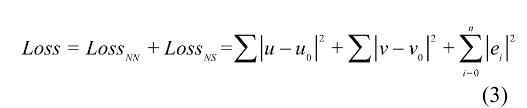
The loss function of either the DBNet or the IncNSNet takes into account of the contributions from both the neural network and the PDE constraints. For example, considering a two-dimensional flow in the IncNSNet, the loss function can be formulated as shown in Eq. (3), where LossNNis the loss corresponding to training variables by the neural network part and LossNSis the contribution from physical constraints of the partial differential equations of the PINN. [u0,v0] is the dataset used to train the network.

For both the DBNet and the IncNSNet, due to the multi-target optimization for training variables and differential equations, the convergence of the loss function is challenging and needs careful treatment. In this work, to forward the training with higher robustness, a modified fully-connected deep learning neural network structure[22]was adopted to enhance the convergence performance. Therein, two transformer networks are introduced to project the inputs to a high-dimensional feature space. A point-wise multiplication is used to update the hidden layers. More details can be found in Ref. [22].

Applications of the DBNet and IncNSNet are presented in the next section. Among these applications, flow simulation (subsection 2.1) refers to acquiring spatial and temporal flow information based on prescribed boundary values, as [u0,v0] shown in Eq. (3). A forward problem or flow inference (subsections 2.2 and 2.3) refers to solving PDEs with deep neural network, including acquiring missing flow information from the known part (for instance,attaining pressure p from known velocity fields or solving the missing velocity field in the domain).Lastly, an inverse problem (subsection 2.4) to identify the parameters in the model equation of a porous media is handled.

2. Results and discussion

2.1 Flow simulation with the DBNet

We first resolve an one-dimensional propagating wave with Gaussian concentration profile using the DBNet. The D1Q3 lattice is employed for the discrete Boltzmann equation. The initial concentration profile,C0, and the exact solution of the corresponding advection-diffusion equation are respectively given in Eq. (4), where μ is the diffusion coefficient.

The particle density distribution fiis trained based on the PINN configuration shown in Fig. 1(a).Comparison between the inferred/simulated and the exact solutions of the above-mentioned problem is given in Fig. 2. Agreement is found for the timedependent concentration profile. It should be noted that we also realized that the accuracy of the DBNet is heavily dependent on parameters such as the Mach number, as there is corresponding constrain from the adopted lattice model.

Fig. 2 (Color online) Simulation of an one-dimensional propagating wave via the DBNet

The canonical lid-driven cavity flow is also considered as a test for the DBNet. The Reynolds number is Re=UL/ν=100, where U is the velocity of the lid, L is the height of the square cavity and ν is the kinematic viscosity. The D2Q9 lattice[27]is adopted for such two-dimensional flow.Velocity components based on the inferred or simulated density distribution fiare obtained and shown in Fig. 3. It can be seen that, the DBNet can deliver reasonable flow structures that is close to the reference flow obtained by traditional CFD simulations. It should be admitted that flow distribution at the top boundary and the bulk area of the vortex structure is underestimated by the DBNet.

Fig. 3 (Color online) Simulation of the lid-driven cavity flow via the DBNet, Re=100

2.2 Inference of laminar flow with the IncNSNet

The above mentioned lid-driven cavity flow is also simulated via the IncNSNet. In the computational domain, random sampling with Latin hypercube scheme is adopted. In Fig. 4, the distributions of velocity components and pressure via IncNSNet show preferable agreement with reference solutions by traditional CFD solver.

Fig. 4 (Color online) Reconstruction of the lid-driven cavity flow by the IncNSNet, Re=100

Furthermore, another case is prepared to explore missing flow dynamics based on the lid-driven cavity problem. Such case is motivated by situations, like in the experimental PIV measurement, in which flow dynamics in certain regions might be missing due to technical reasons. On the other side, the recovery of the missing data is probably necessary or even critical for further flow diagnosis. Here, for the cavity flow, a square region with x～[0.5,0.8] and y～[0.5,0.8],as shown in Fig. 4, is data-missing. Outside of the empty zone, only scattered velocity data is available.The inference of the missing velocity information through the rest zone and the pressure field in the whole domain has been performed by the IncNSNet.The obtained flow distributions of the missing zone are also shown in Fig. 5.

It shows that the flow with higher gradient in vicinity area of the cavity top is inferred precisely.Especially small error in the pressure is observed even without training data of pressure itself. Such case demonstrates the capability of the IncNSNet in flow analysis involving both the inversion and the reconstruction in fluid mechanics.

2.3 Inference of turbulent flow with the IncNSNet

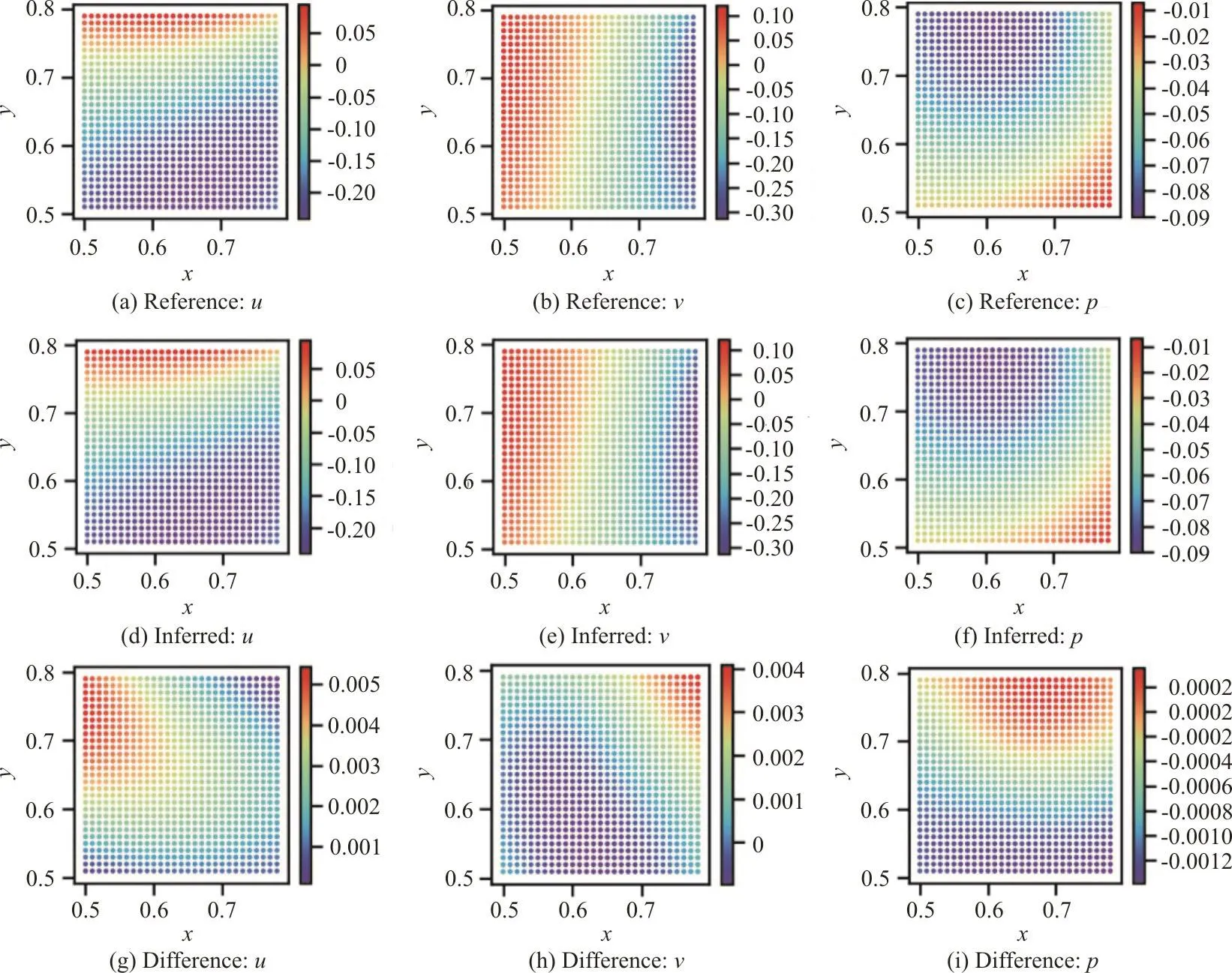
Fig. 5 (Color online) Reconstruction of missing flow information within a lid-driven flow by the IncNSNet: ((a)-(c)) reference flow,((d)-(f)) reconstruted flow using the velocity dataset, ((g)-(i)) error distribution of the inferred results

Fig. 6 (Color online) Reconstruction of turbulent flow within a C-shape tube by the PNS based IncNSNet: ((a)-(c)) reference flow,((d)-(f)) reconstruted flow using the velocity dataset, ((g)-(i)) error distribution of the inferred results

Additionally, a flow passing a bump with Re=1.5×104(Re=UHb/ν, where Hbthe height of the bump) is also investigated with the PNS based IncNSNet. The bump is defined as y=0.05[sin(πx/0.9-π/3）］4, with x～[0.3,1.2]. In this case, flow with much more unsteady characteristics is induced around the bump. The training was completed after sufficient iterations. The reference solution by CFD simulation is shown in the first row of Fig. 7.Due to the curved boundary, there exists an intense velocity variation above the tip and also the shoulders of the bump. The sheltering effect of the streamwise velocity can be observed at the leeside of the bump.Also, there are pressure bumps around the shoulder parts. The inferred flow fields via the PNS based IncNSNet are shown in the second row of Fig. 7. It is demonstrated that the main characteristics of the flow are accurately reproduced. Error distribution in the third row of Fig. 7 shows preferable results in the near region of the bump, while comparatively larger error is found in the downstream for the vertical velocity and pressure.

Eventually, without introducing any specific turbulence models and related turbulence closure training, the PNS based IncNSNet is no longer application-oriented. The Inferred flows show reasonable accordance with the reference ones. This promotes the flexibility in application of machine learning for turbulent flows.

2.4 Inference of flow in porous media with the IncNSNet

To solve the above inverse problem, a modified version of the IncNSNet has been established, as shown in Fig. 8. Firstly, the porosity coefficient n and pressure p in the domain are set as output variables, so that the modified neural network can be established. Secondly, the physics informed part incorporates and takes into account of the porosity effect as a source term (i.e., nvui, with i denoting corresponding velocity components) in the momentum equation, as shown in Fig. 8. Lastly, the IncNSNet training is performed using the velocity data as the training dataset, and the porosity n and pressure p are inferred and outputted.

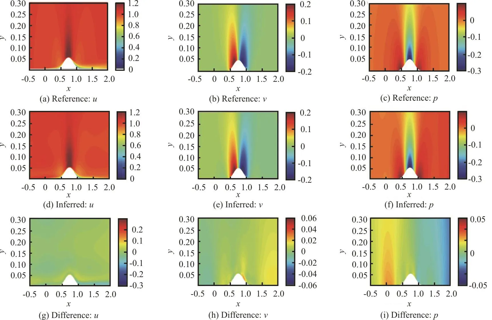
Fig. 7 (Color online) Reconstruction of turbulent flow passing a bump by the PNS based IncNSNet: ((a)-(c)) reference flow,((d)-(f)) reconstruted flow using the velocity dataset, ((g)-(i)) error distribution of the inferred results

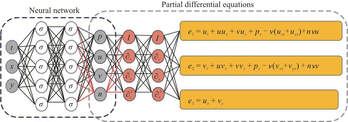
Fig. 8 (Color online) Configuration of the modified IncNSNet for porous zone recognition

3. Conclusions

In this work, we applied two types of PINN,namely the DBNet and the IncNSNet for several flows.The latter one was further extended to parameterised governing system for turbulent flow scenarios. Numerical tests, such as one-dimensional propagating wave,two-dimensional lid-driven laminar flow, turbulent flows within in a C-shape tube and passing a bump,and laminar flow passing through a porous media were considered.

We show that the both the DBNet and the IncNSNet are powerful tools for flow data assimilation and can be successfully used to resolve complex fluid flows, e.g., hydrodynamic problems. The learned results are not only comparably accurate as the traditional CFD techniques, but also indicate considerable capability to reconstruct missing flow dynamics, for both laminar flows and turbulent flows.

Fig. 9 (Color online) Flow passing a porous zone and recognition of the porous zone by the PNS based IncNSNet

With this work, we would like to suggest that more attention should be paid to the machine learning for hydrodynamics. In years to come, the authors hope that machine learning can provide more alternatives in a more intelligent way for vast fluid mechanics applications.

Acknowledgement

This work was supported by the Fundamental Research Funds for the Central Universities of China(Grant No. B200202049).