
The effects of caudal fin deformation on the hydrodynamics of thunniform swimming under self-propulsion *
2020-04-02 03:46YikunFengYuminSuHuanxingLiuYuanyuanSu
水動力學研究與進展 B輯 2020年6期
Yi-kun Feng, Yu-min Su, Huan-xing Liu, Yuan-yuan Su
1. College of Shipbuilding Engineering, Harbin Engineering University, Harbin 150001, China
2. Beijing Institute of Specialized Machinery, Beijing 100081, China
3. Science College, Harbin Engineering University, Harbin 150001, China
Abstract: To investigate the effects of the caudal fin deformation on the hydrodynamic performance of the self-propelled thunniform swimming, we perform fluid-body interaction simulations for a tuna-like swimmer with thunniform kinematics. The 3-D vortices are visualized to reveal the role of the leading-edge vortex (LEV) in the thrust generation. By comparing the swimming velocity of the swimmer with different caudal fin flexure amplitudes fa, it is shown that the acceleration in the starting stage of the swimmer increases with the increase of fa, but its cruising velocity decreases. The results indicate that the caudal fin deformation is beneficial to the fast start but not to the fast cruising of the swimmer. During the entire swimming process, the undulation amplitudes of the lateral velocity and the yawing angular velocity decrease as fa increases. It is found that the formation of an attached LEV on the caudal fin is responsible for generating the low-pressure region on the surface of the caudal fin, which contributes to the thrust.Furthermore, the caudal fin deformation can delay the LEV shedding from the caudal fin, extending the duration of the low pressure on the caudal fin, which will cause the caudal fin to generate a drag-type force over a time period in one swimming cycle and reduce the cruising speed of the swimmer.
Key words: Computational fluid dynamics (CFD) numerical simulation, self-propulsion, caudal fin, deformation
Introduction
In nature, fish can have complex and diverse movements with various fins on their body, such as the fast-start, the periodic cruising, the steering and the hovering. The excellent swimming performances of fish have attracted many researches during the last hundreds of years. The swimming modes of fish are generally divided into two categories: the body and caudal fin (BCF) mode and the median and pair fins(MPFs) mode[1]. The BCF propulsion has five different types: the anguilliform, the sub-carangiform,the carangiform, the thunniform and the ostraciform[2].Only approximately 12% of fish families use the MPF mode as their routine propulsive mode[3].
In this paper, we focus on the thunniform mode of swimming. For a thunniform swimmer, a significant lateral undulation occurs at the posterior 1/3 of the body and the maximum amplitude is reached at the end of the tail peduncle[4]. As the primary swimming mode for many fast fish, the thunniform mode of swimming has attracted a constant attention of scientists. Numerous experimental studies of live fish, focused on the flow field characteristics of the anguilliform, carangiform and thunniform swimmers with the help of the particle image velocimetry (PIV) technology. A double vortex row was observed in anguilliform swimmers[5], in which the wake structure contains two disconnected vortex rings, while in the carangiform and thunniform swimmers one sees a single vortex row with a series of connected vortex rings in the flow field[6]. However,the parameterization experiments based on live fish are either difficult or unfeasible, as it is difficult not only to control the swimming of fish, but also to obtain the transient distribution of the surface pressure of fish[7]. Therefore, a large number of numerical simulations were conducted for the fish swimming.Numerical simulations of fish swimming can be divided into three types: the steady swimming of fish immersed in a uniform incoming flow[6,8-9], the forward swimming of fish with one degree of freedom(1DOF)[10]and the free swimming of fish with three degrees of freedom (3DOF)[11-14]. For the steady swimming, Liu et al.[9]conducted numerical studies of the vortex structures and the hydrodynamic performances of the fish body with interactions between the flexible dorsal, and anal and caudal fins. For the 1DOF forward swimming of fish, Borazjani and Daghooghi[10]simulated the attachment of the leading-edge vortex (LEV), generated by different tails of a mackerel with carangiform kinematics. For the 3DOF self-propelled fish swimming, Kern and Koumoutsakos[11]investigated the hydrodynamics of the anguilliform swimming.
These experimentalal and numerical studies focused on the characteristics of the trailing wake generated by the fish, but without paying enough attention to the features of the LEV of fish, especially the characteristics of the LEV generated by the flexible caudal fin of fish. In this paper we investigate the different effects of rigid and flexible caudal fins on the mechanism of hydrodynamics and 3-D wake structures for self-propelled thunniform swimming,with numerical simulations of a self-propelled tuna-l ike fish body with different caudal fin flexibilities to understand the fundamental physical mechanisms of the hydrodynamic role of the caudal fin’s flexibility and the role of the LEV in the contribution of the pressure distribution on the caudal fin and the force it generates.
1. Materials and methods
1.1 Computation model and kinematics

For the thunniform swimming, the front 2/3 of the swimmer body is too stiff to have undulation and deformation, and the significant lateral movements are observed only at the caudal fin[16]. Therefore, the swimmer body can be divided into three parts: the rigid front body, the flexible rear body and the caudal fin, as shown in Fig. 2. Then, the prescribed kinematics of the swimmer can be divided into two parts: the lateral undulation of the flexible rear body and the heaving-pitching motion of the caudal fin[4].First, the lateral undulation of the flexible rear body is characterized by a backward traveling wave[4],described as

Fig. 1 (Color online) Computational model and two coordinate systems

where y(x,t) is the lateral displacement of the midline, x is the axial position, t is the time, f is the

Fig. 2 (Color online) Multi-joint undulation motion of the swimmer
undulating frequency, k is the wave number, and the amplitude envelope a(x) of the lateral undulation is approximated with a quadratic function[4,8], as denoted in this work as a(x), a quadratic polynomial[4]
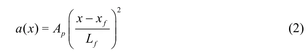
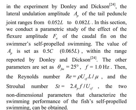
where Apis the lateral undulation amplitude of the tail peduncle joint, xfis the beginning of the flexible rear body and Lfis the length of the flexible rear body.
In this work, to conform with the previous experimental investigation of the “Fangsheng-I”[15]and the other numerical simulations[4,17]in our laboratory, k is set at zero. In addition, the value of our defined k is more conducive to the heaving-pitching motion of the caudal fin, which also makes it convenient to systematically study the effect of the motion parameters of the caudal fin on the hydrodynamic performance of the entire fish. The effect of k on the swimming will be discussed in our future papers.
If we directly use Eq. (1) to define the lateral undulation of the flexible rear body, the body will be elongated during swimming. To address this problem,Li et al.[12]introduced a correction factor in Eq. (1) to ensure that the length of the swimmer remains unchanged. In view of the multi-joint vertebrae of live fish, the flexible rear body is divided into enough segments to emulate the undulation motion and ensure that the body length is unchanged by keeping the length of every segment unchanged during the undulation motion.


Then we use Eq. (4) to determine the rotation motion of each segment Siaround Ji, which can be expressed as:

The caudal fin motion frequency is equal to that of the flexible body’s undulation motion, and the translation motion and the pitch motion have a phase angle φ, which is set to a value of 90°[4,18]. We then have the kinematics of the caudal fin as follows:deformation in the chordwise direction is considered.The deformation profile is determined with an analysis of the effect of the flexure amplitude,described as[18]


1.2 Numerical method
In this work, a 3DOF fluid-body interaction numerical simulation scheme is employed to study the effect of the caudal fin deformation on the selfpropelled swimming. The flow field is simulated using the commercial CFD solver package FLUENT.The FLUENT was successfully used to simulate fish’s self-propelled swimming[19], and the accuracy of the solver was validated extensively for flows with various bionic swimming[4,18,20]. The related validations of this solver can be found in our previous publications[4,18-19]. The governing equations are 3-D viscous incompressible Navier-Stokes equations in a body-fixed coordinate system that is translating with a linear velocity ucand rotating with an angular velocity ω relative to the global coordinate system[21]:
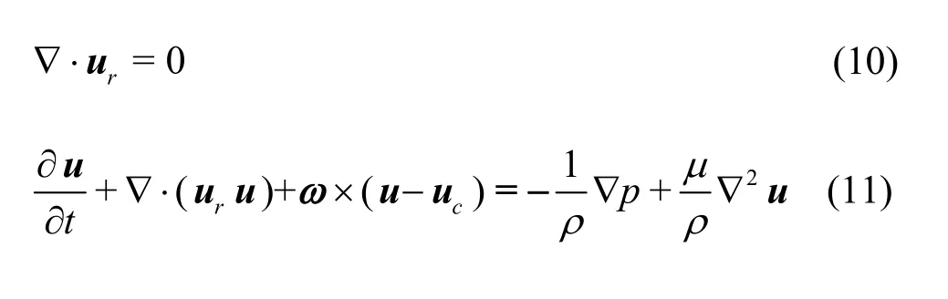
where u is the absolute velocity (the velocity viewed from the global coordinate system), uris the relative velocity (the velocity viewed from the body-fixed coordinate system), ρ is the fluid density, p is the pressure and μ is the dynamic viscosity.
The governing equations Eqs. (10), (11) are discretized using the finite volume method with the pressure-based transient solver. The SIMPLE algorithm is applied for the pressure-velocity coupling,with a first-order implicit discretization in time and a second-order upwind in space. To deal with the flow in a domain with complex 3-D flexible fish moving in prescribed kinematics, the no-slip boundary condition is imposed on the moving boundary:

where r is the position vector from the COM, and is the specified velocity of the deforming motion presented in Section 1.1 in the body-fixed coordinate system.
In the current 3DOF self-propelled swimming,the whole-body motion of the swimmer is computed using the Newton’s motion (momentum) equations:

where m is the swimmer’s mass, UcX, UcYare the components of the translation velocity ucin X, Y directions, respectively, FX,YF are the components of the hydrodynamic force in X, Y directions,respectively, Izis the inertial moment about the yawing axis through the COM,zω is the yawing angular velocity and Mzis the yaw moment. The effect of the inertial and external forces and moments on the swimmer that are independent of the fluid motion, such as the gravitational force, are not considered in this work, similar to other published studies of self-propelled swimming[11-12,19].
During the simulation, FXandYF can be computed by an integral of the local pressure and the viscous forces acting on the swimmer surface[8].


In this work, the swimmer swims in the negative X direction. Therefore, when FXis in the positive X direction (with a positive value), it is considered as the drag type, when FXis in the negative X direction (with a negative value), it is considered as the thrust type. However, whether FXis the drag type or the thrust type, it consists of a pure thrust Tpurand a pure resistance Rpur. In order to separate these two forces, we use the method proposed by Borazjani and Sotiropoulos[8].

where y˙iis the time derivative of the displacement of the swimmer surface, i.e., the velocity of the undulations of the swimmer, in the ith direction.
Then, in order to evaluate the influence of the caudal fin deformation on the swimming efficiency of the swimmer, the Froude efficiencyfη proposed by Tytell[5]is adopted

In this work, the computational domain is an 8.5L(X)×2.0L(Y)×1.0L(Z) cubic tank, which is discretized with a grid including 3.57×10⁶elements.The domain size is tested to be sufficiently large that the influence of the boundary can be ignored. The boundary conditions of the computational domain are set as follows: (1) zero velocity and zero gradient of the pressure on the inlet and far-field boundaries, (2)zero gradient of both the velocity and the pressure on the outlet boundary. The computational domain is divided into three domains: the outer domain (denoted by D1) and two inner domains (denoted by D2 and D3), as illustrated in Fig. 3(a). The swimmer is placed in D2 and D3, specifically, the rigid front body is placed in D2 and the flexible rear body and the caudal fin are placed in D3. The swimmer surface is discretized with triangular elements, and the meshes are sufficiently refined in the regions with a large curvature to ensure the capture of the geometry of the swimmer body and to ensure that the boundary layer is well processed when generating the 3-D meshes. A uniform mesh with constant spacing of 1/60L is used on the interfaces between the inner and outer domains. D2 and D3 are discretized with unstructured tetrahedron meshes, which are locally refined near the surfaces of the swimmer with an element spacing size of 0.0005L to keep the+y values on the swimmer surface from 30 to 150 during the entire swimming process, similar to the approach used by Li et al.[19].The SST k-ω model is applied for the effect of the turbulence, which was fully validated by Leroyer and Visonneau[23]in the simulation of fish’s self-propelled swimming. The mesh size and the growth rate from the surfaces of the swimmer to the boundaries of the inner domains are properly controlled to ensure the quality of the meshes. In D1, the meshes are unstructured in the regions adjacent to D2 and D3, and the other regions are discretized with hexahedral meshes. In addition, the mesh is rapidly stretched in the directions of the swimmer height and width. In the longitudinal direction, the grid stretching is rapid in the upstream region of the swimmer, while in the near wake region the stretching ratio of the mesh is kept below 2% (approximately equal to 1.7%) so as to keep a relatively high streamwise resolution. A combination of smoothing and remeshing is used to regenerate and smooth the meshes inside D2 and D3 after each time-step. The parameters of the smoothing and remeshing approaches are selected reasonably to ensure the quality of meshes.
It can be seen from Fig. 3(a) that with this mesh division strategy, we can well deal with both the undulation motion of the flexible rear body and the flexible deformation of the caudal fin. The flexible deformation of the caudal fin during a quarter cycle is illustrated in Fig. 3(b), where the arrow points to the flexible deformation direction of the caudal fin.
2. Results and discussions


Fig. 3 (Color online) Computational mesh
2.1 Sensitivity study and validation
2.1.1 Sensitivity study
The mesh dependence test is conducted using three meshes with 2.54 (coarse), 3.57 (medium) and 6.79 (fine) million elements. Figure 4(a) shows the time history of Uffor different grids with a time-step size Δt=T/200. It can be seen that the values of Ufcalculated by the medium and fine grids are very close (the calculated value of Ucfof the fine grid is 0.78% larger than that of the medium grid), while the result of the coarse grid is not good.Therefore, we choose the medium grid in all simulations. A sensitivity study of the time-step is also conducted, with Δt={T/400,T/200,T/100} using the medium grid. Figure 4(b) shows the time history of Ucfobtained with different time-steps using the medium gird. It can be seen that with both Δt=T/400, Δt=T /200, reasonable results are obtained and the calculated values of Ucfare in good agreement (the calculated value of Ucfis 0.5%larger at Δt=T /200 than that at Δt=T/400),while with Δt = T/100 the result is not good. Hence,the medium grid and Δt=T/200 are selected in all simulations in this work and the CPU time of one swimming cycle is about 4.5 h in a PC with Intel Core i9-7900x processor and 64 Gigabytes of memory.
2.1.2 Validation


Fig. 4 (Color online) Sensitivity study

Fig. 5 (Color online) Comparison of computed cruising velocity with previous experimental and numerical results for different values of f

The implementation of the fluid-body coupling framework is also validated by the test case of an anguilliform fish undergoes a self-propelled swimming. The length of the fish body is L=1m. In this validation, we use the mesh generation scheme presented in Section 1.2 to generate the numerical grid and the numerical approach presented in Section 1.2 to simulate the flow. The fish geometry is taken from Kern and Koumoutsakos[11]. More details about the fish geometry and the calculation parameters can be found in Kern and Koumoutsakos[11]. The geometry of the resulting 3-D deformed body during the undulation is illustrated in Fig. 6(a). The undulation of the fish is described by the lateral deformation y(s,t)of the midline s of the body, described as


Fig. 6 Validation of a self-propelled anguilliform fish
2.2 Swimming performance
The time history of the forward velocity Uffor different fais illustrated in Fig. 7. It can be observed that the cruising velocity Ucfand the time tcffor the swimmer to reach the cruising state decrease with the increase of fa, as can clearly be seen in Table 1, and Re is in the range of 1.86×10⁶-2.20×10⁶. With the increase of fa, the acceleration of the swimmer’s starting motion increases, that is, the flexible deformation of the caudal fin can provide a larger burst force for the swimmer to start, which becomes larger with the increase of fa. During the cruising state, the Ufslightly fluctuates around the Ucf, as shown in the insets in Fig. 7, where the fluctuations of the Ufare approximately 0.51%, 0.47%, 0.47%, 0.57%, 0.72%and 1.11% for their respective Ucfvalues when favaries from 0 to 0.5.

Fig. 7 (Color online) Time history of the forward velocity Uf for different fa

Table 1 Cruising velocity and time for each swimmer to reach the cruising state
During the self-propelled swimming, the time variations of the lateral velocity Ucyand the yawing angular velocityzω for different faare shown in Figs. 8(a), 9(a), respectively. Figures 8(b) and 9(b)show the time variations of Ucy,zω in one swimming period during the cruising state, respectively. From Figs. 8, 9, we can see that during the entire swimming process, the fluctuation amplitudes of Ucy,zω of a swimmer with a larger faare always smaller than those of a swimmer with smaller fa. These characteristics of Ucy, ωzindicate that the flexible deformation of the caudal fin is conducive to the forward direction stability of the swimmer’s self-propelled swimming.
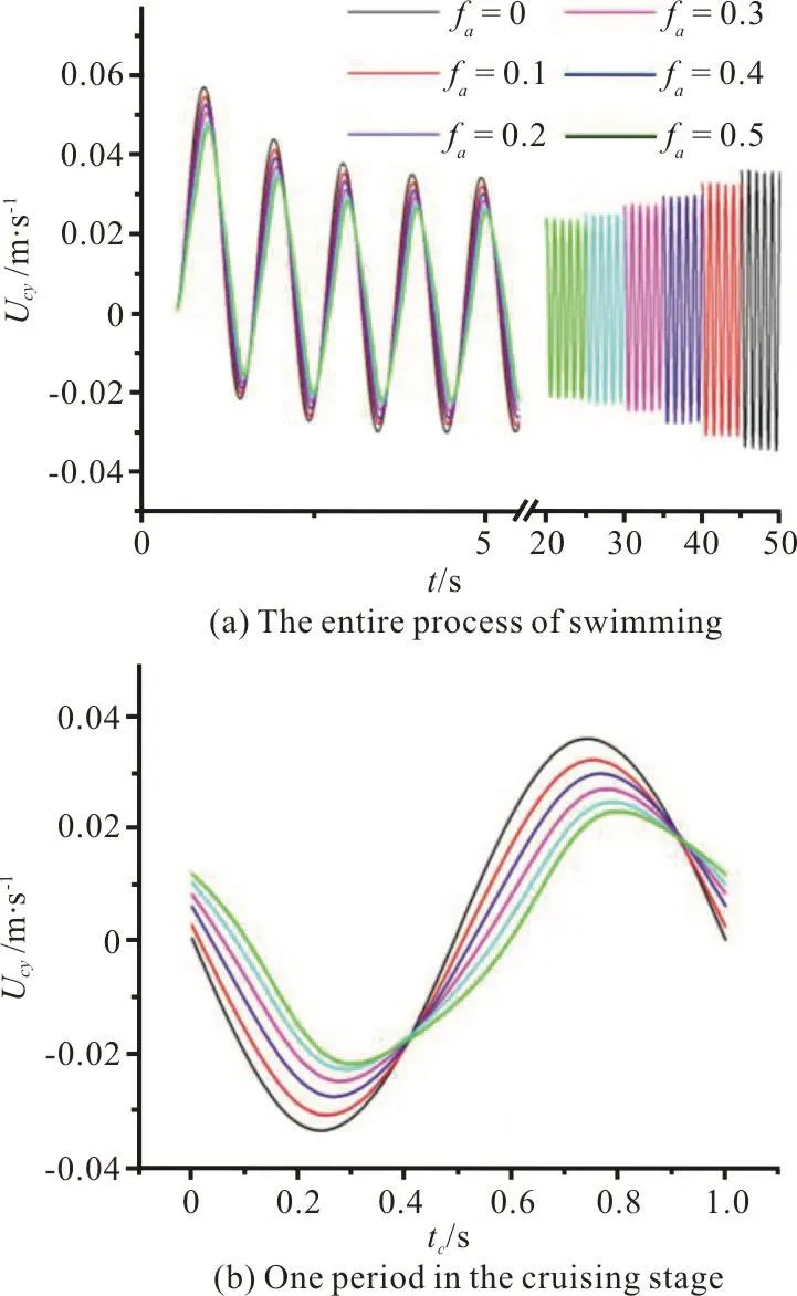
Fig. 8 (Color online) Time history of lateral velocity Ucy for different fa
2.3 Hydrodynamic performance and swimming efficiency


Fig. 9 (Color online) Time history of yawing angular velocity zω for different fa

The cycle-averaged value of the power consumption Phydrofor different fais shown in Fig. 11(a).The cycle-averaged value of Phydrodecreases until it reaches a quasi-steady state for all cases. During the cruising state, the cycle-averaged value of Phydrodecreases firstly as fais raised from 0 to 0.5 with a turning point at 0.3 and then increases as fais further increased. This indicates that the flexible deformation of the caudal fin can have a benefit contribution to the decrease of the power consumption in the cruising state.
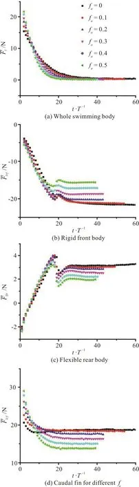
Fig. 10 (Color online) Cycle-averaged value of the longitudinal net force

Fig. 11 (Color online) Power and efficiency
Due to the standard deviation of the Froude efficiencyfη takes a value of an order of 10-3to 10-4in all cases, which is a small quantity of higher order relative to the average value offη. Therefore,we only show the average values offη in Fig. 11(b),and the average values are calculated based on the last five swimming cycles. It can be observed thatfη increases firstly as fais changed from 0 to 0.5 with a turning point at 0.1 and then decreases as fais further increased. The above feature offη indicates that the flexible deformation of the caudal fin can have a beneficial contribution to improve the propulsive efficiency of the swimmer during the cruising state.
2.4 Contribution of the leading-edge vortex to thrust

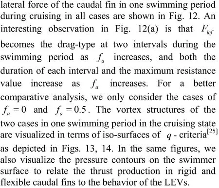

Fig. 12 (Color online) Time history of the hydrodynamic forces of the caudal fin in one cycle in the cruising stage
In the case of fa=0, at the beginning of the cycle (Fig. 13(a)) there are two fully developed LEV tubes (denoted by the vortex V-A in the left column of Fig. 13(a)) attached to the left side surface of the caudal fin, with the whole left side surface of the caudal fin covered by a low pressure region(denoted by LV-Ain the middle column of Fig. 13(a)), and the low pressure is the largest at this instant in the cycle.At this moment, the whole right side surface of the caudal fin is covered by a high pressure region(denoted by H1in the right column of Fig. 13(a)), and the high pressure is the largest at this instant in the cycle. The pressure difference on two sides of the caudal fin contributes to the thrust, this contribution is the largest because the pitch angle of the caudal fin is the largest at this moment. Therefore, the longitudinal net force of the caudal fin reaches a peak value as shown in Fig. 12(a). Due to the pressure difference on two sides of the caudal fin is the largest at this moment, the lateral force of the caudal fin also reaches a peak value as shown in Fig. 12(b).
In the case of fa=0.5, at the beginning of the cycle (Fig. 14(a)) two LEV tubes (denoted by the vortex V-A in the left column of Fig. 14(a)) start to form on the left side surface of the caudal fin. In contrast to the case of fa=0, the vortex V-A is small and only attaches to the leading-edge region of the caudal fin, with a small low-pressure region in front of the caudal fin (denoted by LV-A1in the middle column of Fig. 14(a)). In addition, the right side of the caudal fin also has a small high-pressure region(denoted by H1in the right column of Fig. 14(a)).With the pressure difference on two sides of the caudal fin and the pitch angle of the caudal fin, the longitudinal net force of the caudal fin is in the thrust direction at this moment. However, due to this pressure difference is smaller, the longitudinal net force and the lateral force of the caudal fin are smaller than those in the case of fa=0 (Fig. 12).
At the point of one-quarter cycle in the case of fa=0 (Fig. 13(b)), the size of the vortex V-A is larger but with a weaker strength relative to those at the beginning of the cycle, and the V-A is shed into the wake. At this moment, there are no obvious lowand high-pressure regions on two sides of the caudal fin. The pitch angle of the caudal fin is equal to zero at this time instant, therefore, the pressure difference on two sides of the caudal fin does not contribute to the thrust. Consequently, the longitudinal net force and the lateral force of the caudal fin are close to zero (Fig.12).
At the point of one-quarter cycle in the case of fa=0.5 (Fig. 14(b)), the size of the vortex V-A is larger relative to that at the beginning of the cycle and the whole left side of the caudal fin is covered by the vortex V-A. In contrast to the case of fa=0, the strength of the vortex V-A is larger at two tips of the caudal fin, and the vortex V-A still attaches to the two tips of the caudal fin. Consequently, there are two low-pressure regions (denoted by LV-A2in the middle column of Fig. 14(b)) in the left two tips of the caudal fin. In addition, there are two high-pressure regions in the right two tips of the caudal fin. Because the pitch of the caudal fin is equal to zero, the pressure difference on two sides of the caudal fin does not contribute to the thrust. Therefore, the longitudinal net force of the caudal fin is close to zero (Fig. 12(a)),whereas the lateral force of the caudal fin is not equal to zero (Fig. 12(b)).

Fig. 13 (Color online) 3-D vortex structures visualized with the iso-surfaces of the q-criterion (left column) and the pressure contours on the swimmer surface (middle column and right column) in the case of fa=0 at different instants in the cycle
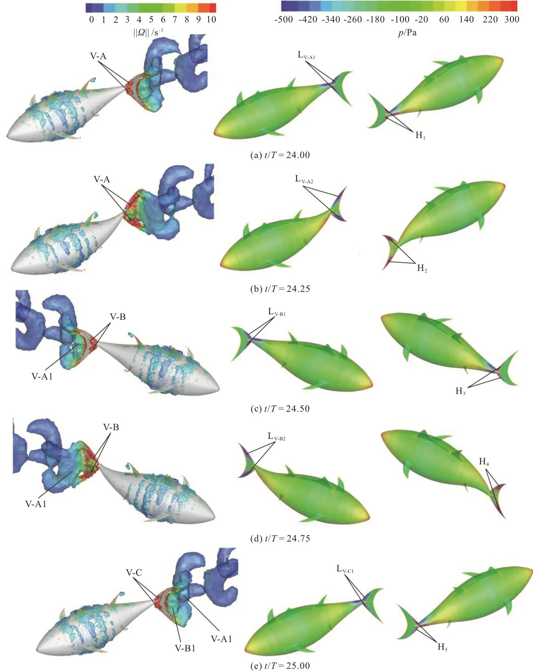
Fig. 14 (Color online) 3-D vortex structures visualized with the iso-surfaces of the q-criterion (left column) and the pressure contours on the surface of the swimmer (middle column and right column) in the case of fa=0.5 at different instants in the cycle
The characteristics of the LEV and the pressure contours of the caudal fin at the point of the half cycle and at the end of the cycle are similar to those at the beginning of the cycle, and are not analyzed here in detail. Only a brief description of the evolution of the LEV in the wake structure is discussed. In both cases of fa=0, fa=0.5, between the points of the quarter and half cycle, the caudal fin flaps leftwards.During this time period, the vortex V-A moves downstream along with the caudal fin surface and eventually merges with the vortex generated by the trailing edge of the caudal fin to form a big TEV(denoted by vortex V-A1 in the left column of Figs.13(c), 14(c)). In addition, there is a new LEV (denoted by vortex V-B in the left column of Figs. 13(c), 14(c))formed at the leading edge of the caudal fin. As the caudal fin continues its motion in the left direction,the vortex V-A1 is seen to deform along with the trailing edge of the caudal fin and is eventually shed from the trailing edge of the caudal fin at the point of three-quarter cycle (the left column of Figs. 13(d),14(d)), with the flapping direction of the caudal fin reversed. At the end of the cycle (Figs. 13(e), 14(e)),we can observe the vortex V-A1 is separated from the caudal fin and moves downstream, the vortex V-B merges with the vortex produced by the trailing edge of the caudal fin and a big TEV is formed (denoted by vortex V-B1 in the left column of Figs. 13(e), 14(e)),with a new LEV (denoted by vortex V-C in the left column of Figs. 13(e), 14(e)) formed at the leading edge of the caudal fin. Finally, comparing the pressure contours on the surface of the swimmer, it should be noted that the most of the thrust is produced by the leading-edge region of the caudal fin due to the contribution of the LEV.
It should be noted that the time for the longitudinal net force and the lateral force of the caudal fin to reach the peak and valley values delays with the increase of fa(Fig. 12). To investigate the mechanism of this phenomenon, we plot the vortex structures along with the pressure contours on the surface of the swimmer at instants corresponding to the peak and the valley of the longitudinal net force of the caudal fin in the case of fa=0.5, as shown in Fig. 15. As shown in Fig. 15(a), in contrast to the case at the beginning of the cycle, the whole left side of the caudal fin is covered by the vortex V-A, leading to a larger low-pressure region in the left side of the caudal fin, and at the same time, the right side surface of the caudal fin is covered by a larger high-pressure region.Apparently, the pressure difference on two sides of the caudal fin at this instant is larger than that of the caudal fin at the beginning of the cycle. The angle that the caudal fin makes with the swimming direction(denoted by θ) is shown in the inset in Fig. 15(a),this angle makes the components of the force acting on the caudal fin larger both in the swimming and lateral directions. Consequently, both the longitudinal net force and the lateral force of the caudal fin reach the peak values at this instant (Fig. 12). As shown in Fig. 15(b), similar to the case at one-quarter cycle, the vortex V-A is still attached to the two tips of the caudal fin, leading to a low-pressure region LV-A2on the left side of the back half of the caudal fin, which contributes to the drag. In contrast to the case at one-quarter cycle, the vortex V-B starts to be formed on the right side of the leading edge of the caudal fin,to generate a low-pressure region LV-B1on the right side of the front half of the caudal fin, which contributes to the thrust. Comparing LV-A2and LV-B1in the middle and right columns of Fig. 15(b), it can be observed that the drag generated by LV-A2is larger than the thrust generated by LV-B1. Therefore, the longitudinal net force of the caudal fin is in the negative swimming direction. Considering the angle that the caudal fin makes with the swimming direction(denoted by θ), the lateral force of the caudal fin is small in the left direction of the swimmer. Finally,comparing the vortex dynamics generated by the caudal fin, it should be noted that the flexible deformation of the caudal fin can lengthen the duration of the attachment of the LEV on the caudal fin.
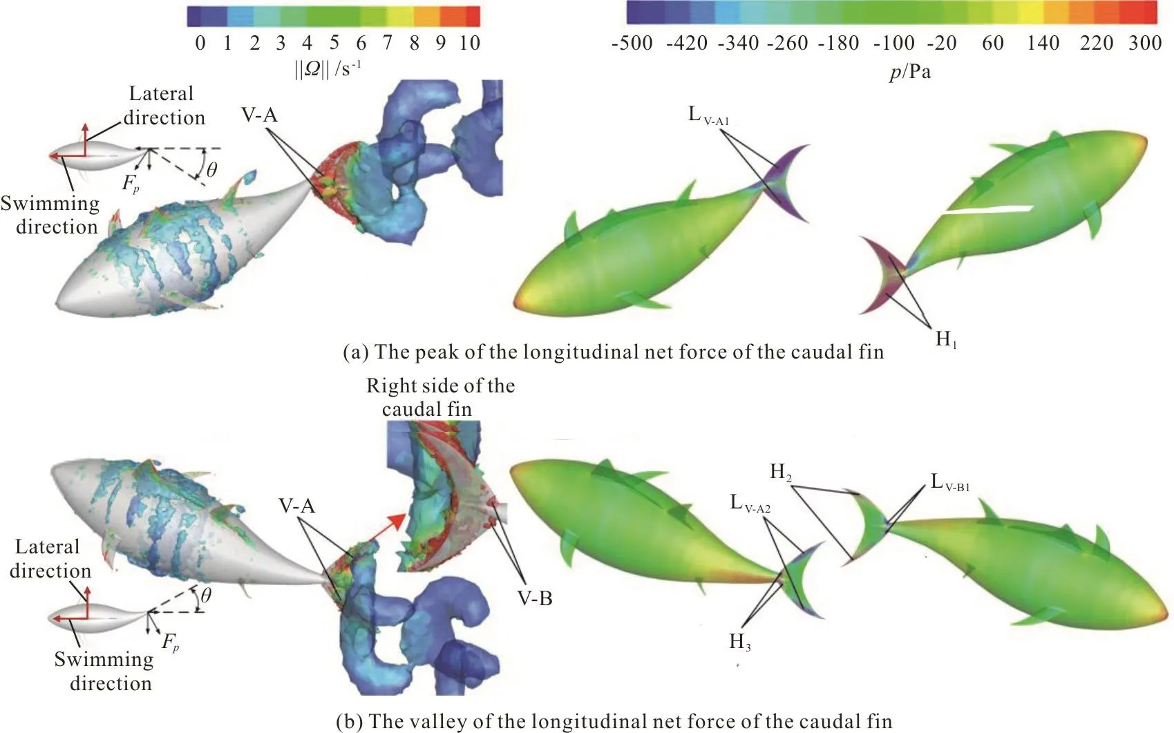
Fig. 15 (Color online) 3-D vortex structures visualized with the iso-surfaces of the q-criterion (left column) and the pressure contours on the surface of the swimmer (middle column and right column) in the case of fa =0.5
3. Conclusions
In this study, numerical simulations are carried out for the effects of the caudal fin deformation on the hydrodynamics of a self-propelled thunniform swimmer. The complex interaction of the swimmer with the fluid is analyzed by an in-house UDF program linked to the main code of the commercial flow solver FLUENT based on the fluid-body interaction method.
Our results show that the starting acceleration of the swimmer increases with the increase of the flexure amplitude faof the caudal fin, indicating that the caudal fin deformation can provide a larger burst force for the swimmer to begin swimming, and this burst force becomes larger with the increase of fa. On the contrary, Ucfdecreases with the increase of fa.Therefore, the flexible deformation of the caudal fin contributes to the rapid start of the swimmer, but is not conducive to the high-speed cruising of the swimmer. The fluctuations of Ucyandzω during the entire swimming process decrease with the increase of fa, that is, the caudal fin deformation is beneficial to the forward direction stability of the swimmer.
By analyzing the hydrodynamic forces of different parts of the swimmer, it is found that the caudal fin is the main propulsive part of the swimmer and that the remaining moving part of the swimmer’s body can also produce a thrust, but its contribution is smaller than that of the caudal fin. During the starting stage, the cycle-averaged value of Flcfmonotonically increases with the increase of fa. However,during the cruising stage, the cycle-averaged value of Flcfmonotonically decreases with the increase of fa.The swimming efficiency of the swimmer with different fais evaluated using the Froude propulsive efficiency, the results show that the flexible deformation of the caudal fin can have a beneficial contribution to improve the propulsive efficiency in the cruising state.
Detailed analyses of the pressure field and the vortex dynamics indicate that the formation and the attachment of the LEV on the caudal fin are responsible for the generation of the thrust. The pressure contours on the swimmer surface show that the most of the thrust is produced by the leading-edge region of the caudal fin due to the attachment of the LEV. In addition, comparing the vortex structures generated by caudal fins with different fa, it is found that the caudal fin deformation can delay the shedding of the LEV from the caudal fin and extend the duration of the low pressure on the caudal fin. During the cruising stage, the delayed shedding of the LEV makes the caudal fin generate a drag-type force over a period in one swimming period, which reduces the cruising speed of the swimmer.

- 水動力學研究與進展 B輯的其它文章
- Control of water contamination on side window of road vehicles by A-pillar section parameter optimization *
- Numerical simulation of the effect of waves on cavity dynamics for oblique water entry of a cylinder *
- Reduction of wave impact on seashore as well as seawall by floating structure and bottom topography *
- Applying physics informed neural network for flow data assimilation *
- Experimental analysis of tip vortex cavitation mitigation by controlled surface roughness *
- Numerical simulations of propeller cavitation flows based on OpenFOAM *