
Diffusion with a Discontinuous Potential: a Non-Linear Semigroup Approach
2021-06-29 02:15YongJungKimandMarshallSlemrod
Yong-Jung Kimand Marshall Slemrod
1 Department of Mathematical Sciences,KAIST,291 Daehak-ro,Yuseong-gu,Daejeon 305-701,Korea
2 Department of Mathematics,University of Wisconsin,Madison WI 53706,USA
Abstract. This paper studies existence of mild solution to a sharp cut off model for contact driven tumor growth. Analysis is based on application of the Crandall-Liggett theorem for ω-quasi-contractive semigroups on the Banach space L1(Ω).Furthermore,numerical computations are provided which compare the sharp cut off model with the tumor growth model of Perthame,Quir′os,and V′azquez[13].
Key Words: Nonlinear semigroups,tumor growth models,Hele-Shaw diffusion.
1 Introduction
In their paper [13], Perthame, Quir′os, and V′azquez proposed the following model for tumor growth

wherevis the cell density,v0is the initial value,andpis the pressure field.In their model,the pressure field is approximated by

where the coefficientvcis the maximum packing density and is set tovc= 1 for convenience. In this case,Eq.(1.1)is written as

The contact driven tumor growth model is taken as limitm →∞of (1.3). Perthame,Quir′os,and V′azquez[13]proved that,if the initial value is smooth and bounded

the pair(vm,pm)converges to(v∞,p∞)asm →∞which satisfy a Hele-Shaw type diffusion model

in the sense of distributions. Furthermore,

and

where the inclusion relation(1.6)is given by the set-valued function

Note that the diffusion term in (1.5) is present only whenv∞= 1. Indeed, the limiting case gives an extreme scenario that the domain is divided into two parts, specifically when(a)the diffusion does not appear at all or(b)it is concentrated atv=1.
We note the Hele-Shaw diffusion equation,(1.5)-(1.7),cannot be used as a model for the limiting case. First, it does not single out a solution(though to be fair the extended version of (3.1a) that we introduce in Section 3 will also be defined by an inclusion relation). The main reason is that the set-valued functionP∞(v) has discontinuity at the stable steady state of the reaction term,v= 1. Furthermore, if the initial value is not bounded by (1.4), the solution is not defined. As an alternative system, we consider a sharp cut off model

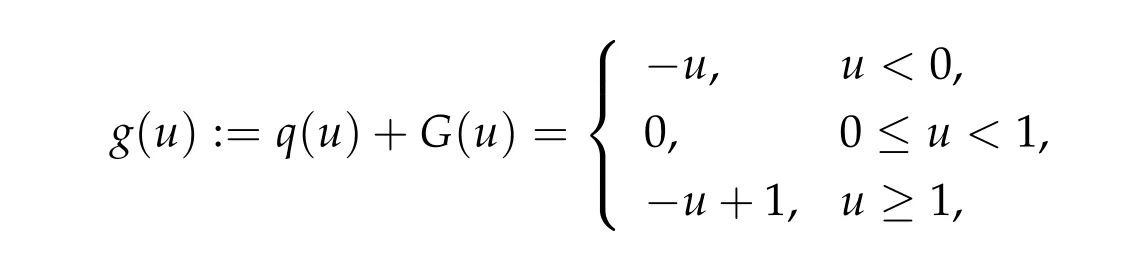
where

which has been introduced by Kim and Pan[11]. We setG(1)=1 in(1.9a)to connect the model to the nonlinear diffusion in(1.3)which has the same property,i.e.,vm= 1 whenv=1.The value of the potential at the discontinuity pointu=1 makes a difference since it is a stable steady state of the reaction functionf(u).
Kim and Pan suggested that the cut off model(1.8)-(1.9b)provides an alternative to(1.3)-(1.4)withm ?1 large. To check their conjecture Kim and Pan performed numerical experiments and their results are here illustrated in Fig.1 of Section 4. We observe that that numerical results for(1.3)withmlarge and(1.8)-(1.9b)are almost identical.
The apparent success of the Kim-Pan model of course raises the mathematical issue as to existence of solutions to (1.8)-(1.9b) for appropriately given initial and boundary conditions. To address this issue we will place the problem within the context of nonlinear semigroups ofω-quasi-contractions on the Banach spaceL1(Ω). The advantage of this formulation is obvious: we will only need use of the existing mathematical theory as provided by the classical Crandall-Liggett theorem[6].
This paper has three sections after this Introduction. Section 2 provides a review of the theory ofm-accretive operators and non-linear semigroup theory on Banach spaces.Section 3 applies this theory to obtain the existence of mild solution to system(1.8)-(1.9b).Section 4 gives careful comparisons of numerical solutions of (1.3) and (1.8)-(1.9b). In particular,we observed there is nice convergence solutions of(1.3)to a solution of(1.8)-(1.9b)when the CFL condition is satisfied. However,when the CFL condition is violated,solutions of(1.3)blow up where as solutions of(1.8)-(1.9b)remain bounded albeit with oscillations.
2 Review of m-accretive operators and non-linear semigroups
We follow the presentations of Evans [9] and Barbu [1] though the definitions are standard(also see[2,12]). Let X be a Banach space with norm‖·‖. An operatorA:D(A)→X with its domainD(A)?X is called accretive if

for allu,v ∈D(A) andλ ∈R+. If, in addition,Range(I+λA) = X for some(equivalently for all)λ>0,thenAis calledm-accretive. A simple way to check accretiveness in examples is to define
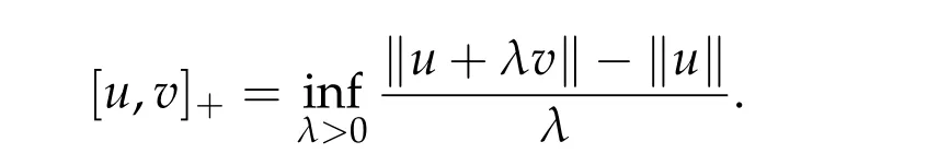
Then the operatorAis accretive if and only if

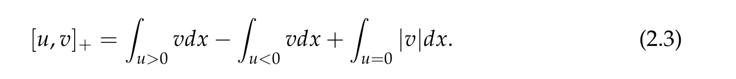
When X=L1(Ω)for a bounded domain Ω?Rn,we may use the result of Sato[14]:
We are interested in resolving the initial value problem

whereAis anm-accretive set-valued operator.
In their classic paper, Crandall and Liggett [6] provided a mild solution to (2.4a),(2.4b)via a sequence of discrete problems where the time derivative in(2.4a)is replaced by a difference quotient:

forε> 0 small so that(2.4b),(2.5)can be solved recursively. We summarize their results as follows.
IfC ?X,a semigroup onCis a functionSon[0,∞)such thatS(t)mapsCintoCfor eacht ≥0 and satisfies
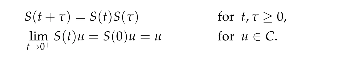
IfSis a semigroup onCand there is a real numberωso that

fort ≥0 andu,v ∈C,we say the semigroup isω-quasi-contractive.

We callu(t) :=S(t)u0a mild solution of(2.4a),(2.4b).
In general, we do not know thatD(A) is invariant under the mapS(t) (unlike the case of linear semigroups whereu(t) =S(t)u0,u0∈D(A), provides a strong solution of (2.4a), (2.4b), see e.g., [10]). However, there is a generalized domain ?D(A) defined by Crandall [7], which is invariant underS(t). In particular,S(t)u0is locally Lipschitz continuous int,u0∈?D(A).
In the initial-boundary value problem of Section 3, we will be interested in the case of X=L1(Ω)and thus the nonlinear semigroup theory for reflexive Banach spaces does not apply(see for example Barbu[1],Evans[8,9],and Zeidler[15]).
3 Existence
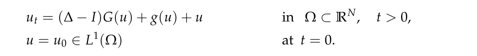
We consider the initial-boundary value problem

where Ω is a bounded open set in RNwith a smooth boundary. Here,

Note

and hence?g(u)=u ?f(u)has a monotone increasing graph. Next,note
and hence?g(u)is continuous on R with a monotone graph. Thus

and we can rewrite(2.1),(2.2)as
Next,we recall two results given by Br′ezis-Strauss[3]and Barbu[1].
Proposition 3.1.LetXbe a real Banach space, A an m-accretive operator,and B a continuous m-accretive operator with D(B)=X. Then, A+B is m-accretive.
Proposition 3.2(Barbu[1],p.114).LetX=L1(Ω). Define the operator
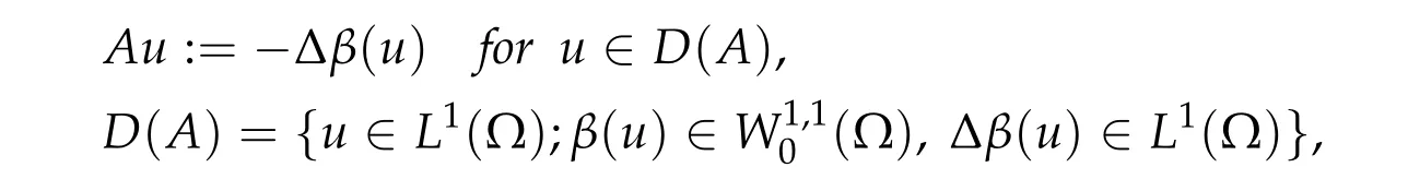
where β is a maximum monotone graph inR×Rwith0∈β(0)andΩis an open bounded subset ofRN with smooth boundary. Then,the operator A is m-accretive in L1(Ω)×L1(Ω).
Lemma 3.1.The map ?g:R→Ris continuous and m-accretive on L1(Ω).
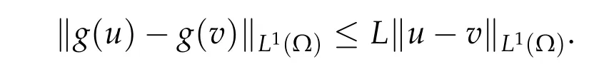
Proof.The map?g: R→R is globally Lipschitz continuous:|g(u)?g(v)|≤L|u ?v|.This implies
Furthermore,Sato’s lemma of Section 2 implies?g:L1(Ω)→L1(Ω)is accretive.Finally,the range conditionu+λg(u) =f,f ∈L1(Ω) is satisfied by solving this equation for eachu:
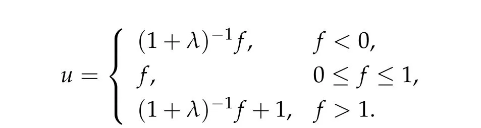
Clearly,f ∈L1(Ω)impliesu ∈L1(Ω).
Lemma 3.2.The operator A1defined by

is m-accretive on L1(Ω)where

Proof.Use Proposition 3.1,Proposition 3.2,and Lemma 3.1.
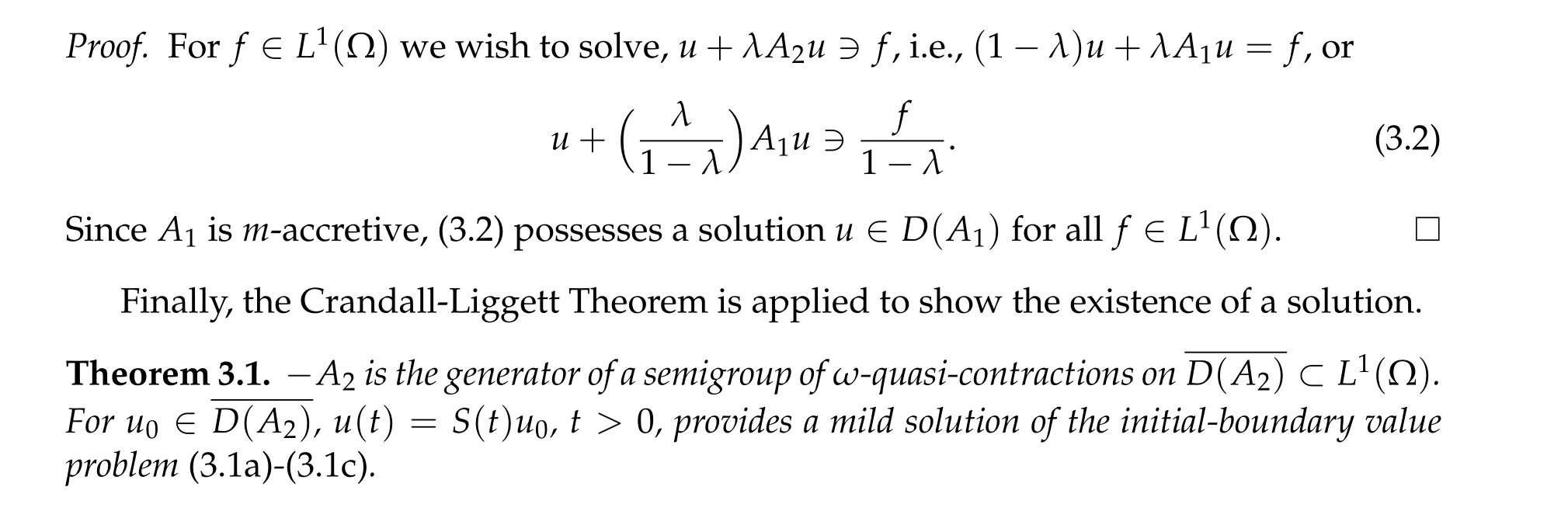
Lemma 3.3.The operator A2:=A1?I,D(A2)=D(A1),satisfies the range condition R(I+λA2)=L1(Ω)for λ>0,sufficiently small.
4 Numerical simulations
The heat and the Poisson equations are often used as canonical systems to test numerical schemes. In the theory, uniform ellipticity and bounded diffusivity are assumed. However, the diffusion model with a discontinuous potential is an extreme case where both assumptions fail. The behavior of numerical schemes for such discontinuous diffusion models is not usually studied. An explicit finite difference scheme, a forward in time and centered in space scheme (see Appendix), is considered in this section which gives characteristic properties of related numerical schemes in this simple context.
We first test if the numerical solution of

gives the same subsequential limit of

which has been obtained by Perthame et al. [13]. Here,pm,G, andfare respectively given by (1.2), (1.9a), and (1.9b). The two model equations are solved numerically and compared in Fig.1. The computation is done on a domain Ω = [?10,10] with the zero Dirichlet boundary condition. The initial values are

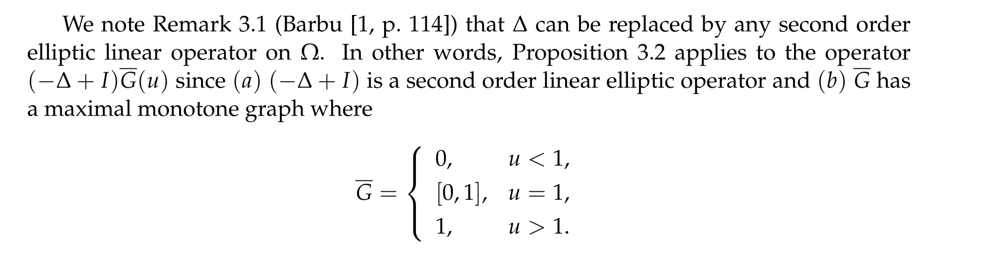
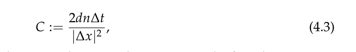
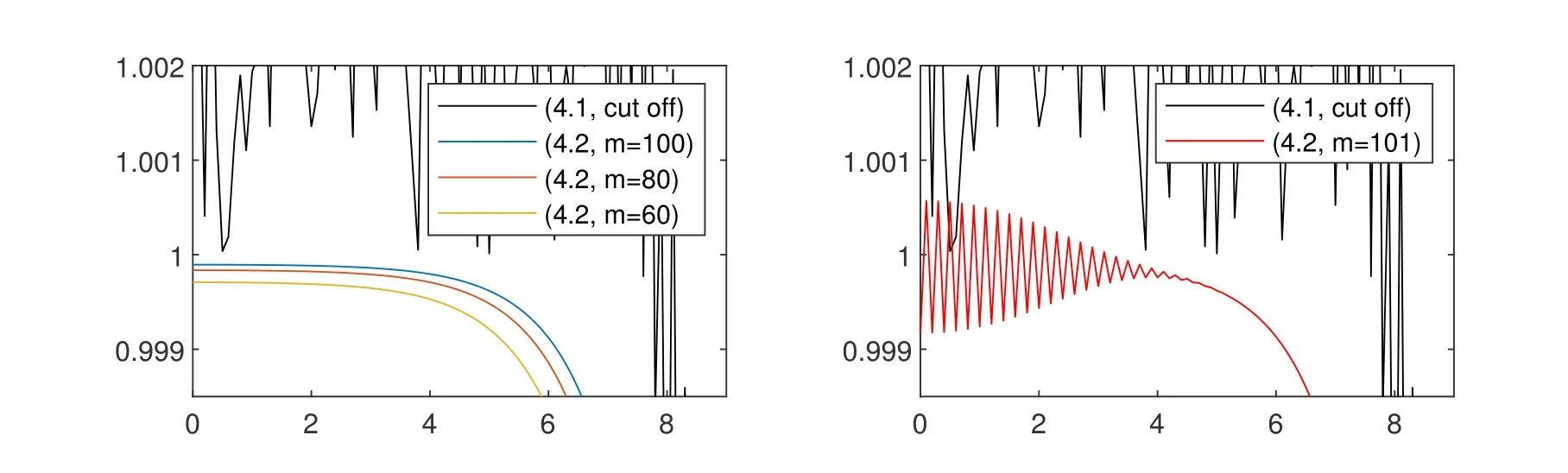
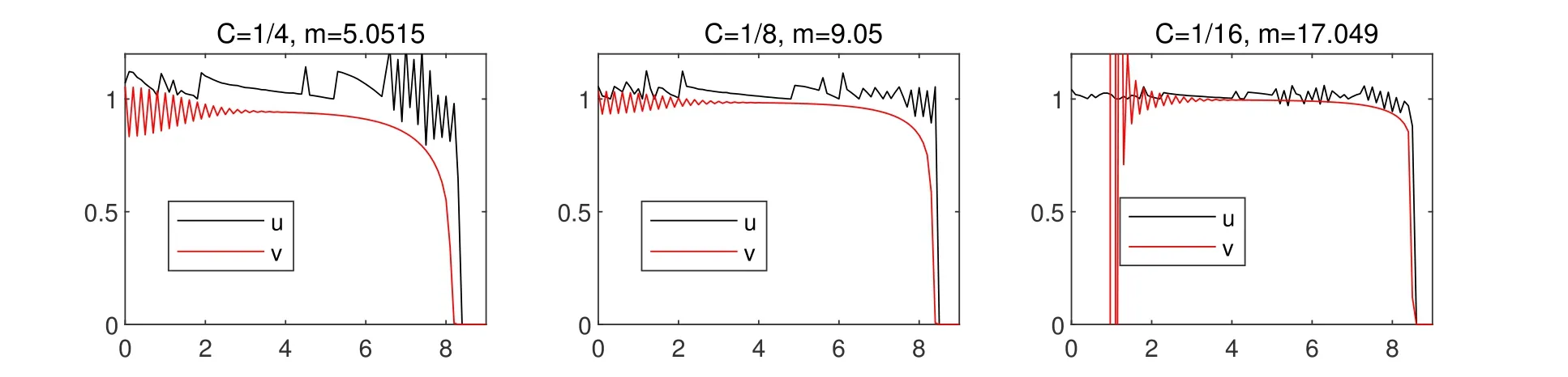
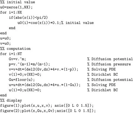
and zero otherwise. The solution is symmetric with respect tox=0 and hence displayed only on the domain 0 An explicit numerical scheme for a partial differential equation of an advection phenomenon should satisfy the CFL condition, i.e., the Courant numberCshould be less than one,i.e., wheres> 0 is the speed of the advection phenomenon, Δxis the space mesh size, and Δtis the time step. The Courant number of a numerical scheme for a parabolic problem is given by whered>0 is the diffusivity andn ≥1 is the space dimension. In the first three numerical computations,we take time and space meshes with The diffusivity of the continuous diffusion model(4.2)isd=mvm?1. Hence,if the mesh size is given by(4.4),the Courant number is bounded by where the inequality comes from the solution bound|v|≤1. The Courant number for the discontinuous diffusion model(4.1)is In Fig.1,snap shots of numerical solutions of the two models are given att=10. See Appendix??for the matlab code of this computation. Solutions of(4.2)clearly converge to the solution of the cut off model(4.1)asm →∞. This convergence is monotone and convinces us that the solution of the cut off model(4.1)is the limit of Perthame et al.[13]that satisfies the Hele-Shaw diffusion equation,(1.5)-(1.7). In Fig.2,the cell density and the diffusion pressure for the two models are compared whenm= 100. The figure in the right shows that the diffusion pressurepmof the continuous model(4.2)connects the interface and inside cells monotonically. This profile is consistent in time and propagates with the front without changing its shape.On the other hand, the potentialGof the discontinuous model (4.1), which also plays the role of the pressure,oscillates as in the figure in the left. The position and size of the oscillating region varies as the solution propagates. However,the inconsistent behavior is completely averaged out and the cell growth interfaces of the two models agree perfectly. Figure 1: Snap shots of (4.1) and (4.2) at t=10. Mesh sizes are Δx =0.1 and Δt=5×10?5. Figure 2: Snap shots of cell density and potential for (4.1) and (4.2). We took m=100 and t=10. In Fig. 3, we observe numerically what happens when the CFL condition fails. The Courant number for the numerical solution of the continuous diffusion model (4.2) isCv=m×10?2when the mesh is given by (4.4). Hence, the CFL condition fails ifm>100, which is why we did the computation form ≤100 in Fig. 1. Indeed, ifm= 102,the numerical solution blows up and becomes unbounded in a finite time. In the right of Fig. 1, the numerical solutions are magnified for values between 0.9 and 1.2. One can see that the numerical solution of the discontinuous cut off model oscillates. This is because of the discontinuity of the diffusion potentialGand the fact thatu=1 is a stable steady state. Note that even a small numerical error near the steady stateu= 1 gives large oscillating noise in ΔG(u)due to the discontinuity of the potentialGand produces the oscillation. We can also see that the solution of the cut off model (4.1) stays above other solutions. To see this more clearly, the solutions are magnified near the steady stateu= 1 in Fig. 3. See the figure in the left and find that numerical solutions for the nonlinear diffusion model(4.2)increase asmincreases and stay below the solution of the sharp cut off model (4.1). However, even the solution of the nonlinear diffusion model oscillates whenm= 101, i.e., when the CFL condition fails (see the figure in the right).The solution of the discontinuous model(4.1)is not an upper bound of the solution of the continuous model(4.2)anymore. Ifm=102,the solution blows up entirely and becomes unbounded. In Fig.4,three snap shots of the numerical solution of the cut off model(4.1)are given Figure 3: Magnified snap shots of (4.1) and (4.2) at t=10. Figure 4: Snap shots of (4.1) at t=10. We took Δx =0.1 fixed and Δt=0.005,0.0013, and 0.00033 from left. with different Courant numbers. The space mesh size is taken with Δx= 0.1 and three different time mesh sizes taken with Notice that the Courant numberCuin(4.5)is not defined sinceG′(u) = ∞whenu= 1.The Courant number denoted in Fig.4 is the one for the constant diffusivity case given in(4.3)withd= 1 andn= 1. We observe that the solution oscillates with any Courant number. However, the solution is numerically stable as long as the Courant number is less than one,i.e.,if the CFL condition for a constant diffusivity case is satisfied. IfC>1,both numerical solutions of the discontinuous diffusion model(4.1)and of the constant diffusivity one blow up together. It is unexpected that the discontinuous diffusion model(4.1)is more stable than the continuous nonlinear diffusion model(4.2). In Fig.5,we observe that the blowup behavior of the continuous diffusion model(4.2)is consistent. We take Δx=0.1 fixed and three cases of In these three cases, the Courant numbers of the unit diffusivity cases are respectivelyC= 4?1, 8?1, and 16?1. Numerical solutions of the cut off model (4.1) are denoted byuin the figures. The numerical solutions of the continuous model (4.2) are given with borderline exponentsmwhich makes a solution about to blow up. We may observe that thesem×C1,i.e.,Cv1. Figure 5: Snap shots of (4.1) and (4.2) at t=10. Δx =0.1 and Δt=0.0013,0.00065 and 0.00033 from left. The diffusion equation(1.8)with a discontinuous diffusion potentialGcan be used as a simplified model for contact driven tumor growth[13],finite time extinction[5],obstacle problems [4], and etc. However, since most theories of parabolic and elliptic problems are based on bounded diffusivity, such equations are rarely studied. In this paper we demonstrated that nonlinear semigroup theory is applicable to such extreme cases and obtained the existence of a mild solution.We also found that a numerical scheme applied to a discontinuous diffusion model (4.1) is more stable than expected. It surprisingly gives the correct interface of tumor growth even when the numerical solution for the continuous diffusion model(4.2)blows up. Appendix: Numerical computation code The numerical computations in this paper are based on a matlab code in the below. We have computed the solution changing the parametermand time step sizedt, and then displayed them as in figures. Acknowledgements This work was supported in part by National Research Foundation of Korea (NRF-2017R1A2B2010398). The authors thank Profs. L.C.Evans and W.Strauss for their valuable suggestions.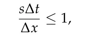


5 Conclusions

 Analysis in Theory and Applications2021年2期
- Analysis in Theory and Applications的其它文章
- Classification of Positive Ground State Solutions with Different Morse Indices for Nonlinear N-Coupled Schr¨odinger System
- Ground States to the Generalized Nonlinear Schrdinger Equations with Bernstein Symbols
- Index Iteration Theory for Brake Orbit Type Solutions and Applications
- Deformation Argument under PSP Condition and Applications
- Multiple Sign-Changing Solutions for Quasilinear Equations of Bounded Quasilinearity
- Ground States to the Generalized Nonlinear Schr¨odinger Equations with Bernstein Symbols