
A fast convergence fourth-order Vlasov model for Hall thruster ionization oscillation analyses
2022-03-10 03:50ZhexuWANGReiKAWASHIMAandKimiyaKOMURASAKI
Plasma Science and Technology 2022年2期
Zhexu WANG,Rei KAWASHIMA and Kimiya KOMURASAKI
The University of Tokyo,7-3-1,Hongo,Bunkyo,Tokyo 113-8656,Japan
Abstract A 1D1V hybrid Vlasov-fluid model was developed for this study to elucidate discharge current oscillations of Hall thrusters(HTs).The Vlasov equation for ions velocity distribution function with ionization source term is solved using a constrained interpolation profile conservative semi-Lagrangian method.The fourth-order weighted essentially non-oscillatory(4th WENO)limiter is applied to the first derivative value to minimize numerical oscillation in the discharge oscillation analyses.The fourth-order accuracy is verified through a 1D scalar test case.Nonoscillatory and high-resolution features of the Vlasov model are confirmed by simulating the test cases of the Vlasov-Poisson system and by comparing the results with a particle-in-cell(PIC)method.A 1D1V HT simulation is performed through the hybrid Vlasov model.The ionization oscillation is analyzed.The oscillation amplitude and plasma density are compared with those obtained from a hybrid PIC method.The comparison indicates that the hybrid Vlasov-fluid model yields noiseless results and that the steady-state waveform is calculable in a short time period.
Keywords:Hall thruster,ionization oscillation,Vlasov equation,semi-Lagrangian method
Nomenclature
Abbreviations
1.Introduction
A HT,a widely used EP device used for spacecraft propulsion[1],employs a cross-field configuration with a radial magnetic field and an axial electric field,where electrons are trapped and move in theE×Bdirection.This configuration generates efficient ionization within a short discharge channel.An electric field is maintained to accelerate the ions to provide the propulsion.Although many successful applications of HTs and other Hall plasma sources have been reported,much of their physics remains poorly understood[2].
One important issue of HT is the discharge current oscillations.Several types of fluctuations are existed in the HT with a widely range of frequency band[3-7].These fluctuations are closely related to the performance and plasma characteristics of HTs.For plasma sources,the fluctuation with the largest discharge amplitude observed is the ionization oscillation.In HT,ionization oscillation is also called the breathing mode,which has a strong effect on the power processing unit.The beathing mode typically has a frequency in the rage of 10-30 kHz,and its physical process is often described by using the predator-prey model[8].Once a frequent ionization occurs in the discharge channel,the ion number density grows in this region while the propellant neutral particles are consumed.When the neutral particles are depleted,the ionization rate becomes small and most of the ions are exhausted from the channel.The propellant neutrals replenish the channel again and the next cycle of ionization begins.Such periodic oscillation has been demonstrated through experimentation[4]and numerical simulation[5].A deep understanding of the physics and accurate numerical modelling of the oscillations in HTs are fundamentally important for the further development of high-performance plasma devices[3,6,9].
Several numerical models have been developed for solving the plasma behaviours in HTs.An early work employed full PIC model was presented by Szabo[10],he investigated the thruster performance of a thruster-with-anode and optimized the magnetic field topology;Cho[11]used the full PIC model to simulate a UT-SPT-62 type thruster and compared the results of wall erosion with experiment.Hybrid PIC-fluid models that treat heavy species kinetically and electrons as a continuum fluid are also widely used,the a very pioneer work was conducted by Komurasaki[12],the basic plasma behaviours and ion loss to the wall were studied;Kawashima[5]combined the PIC model with hyperbolic electron fluid model and successfully reproduced the rotation spoke in azimuthal direction.One disadvantage of the particle model is the statistical noise which is generated due to the finite number of macroparticles handled in the simulation[13].For the analyses of plasma fluctuation,these numerical noises might interfere with physical oscillations,leading to an inaccurate conclusion.
An alternative approach to the PIC model is the Eulertian type Vlasov model[14,15],which can be solved through SL method[16,17].SL method is a grid-based method which is developed to solve the linear advection equation.The noise caused by the finite number of macroparticles in the PIC method can be eliminated by changing to the SL method because it solves the IVDF under Eulerian framework.Furthermore,the high-order WENO scheme can be employed to reduce the numerical diffusion and keep the stability during simulation.
As described herein,a noiseless hybrid Vlasov-fluid model was developed to study the discharge current oscillation in HT.The flows of ions and neutral particles are modelled through the Vlasov equation with an ionization source term,where the electrons are assumed as fluid.Highorder schemes are desired for accurate simulation of discharge current oscillations with short wavelengths.Fourth-order spatial accuracy is achieved in the Vlasov equation solver and verified using a simple test problem.In addition,the noiseless feature of the solver is demonstrated through a two-stream instability problem.Finally,the Vlasov equation solver is coupled with the magnetized electron fluid model,and the discharge current oscillation phenomenon is simulated.
2.Physical model and numerical method
2.1.Kinetic model of ion dynamics for the HT simulation
For one-dimensional(1D)simulation of the HT discharge,a kinetic-fluid hybrid model[18]is used for this study.In this model,the flows of ions and neutral atoms are modelled using the Vlasov equation,where the electron flow is assumed as fluid.
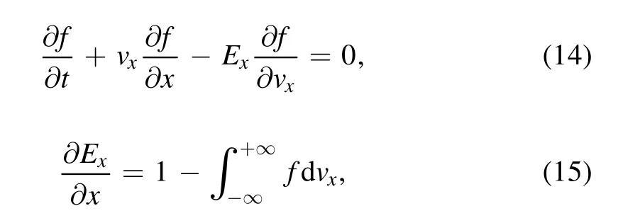
The 1D1V kinetic model includes one dimension in space and one dimension in velocity,where the ions are treated as non-magnetized particles.In the numerical scheme mentioned in this paper,the ionization process and advection process are solved separately,the ionization process follows:

and the advection process is generated by the Vlasov equation:
For the simplification of the equation set,the Vlasov equation for ions with ionization source terms reads:

and the advection process of neutral particles follows:
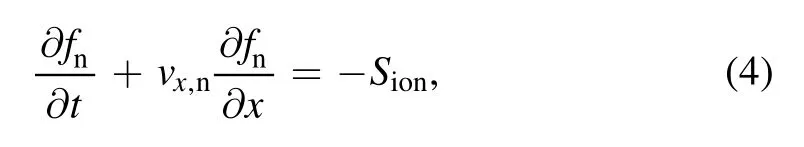
hereExrepresents thex-electric field,estands for the elementary charge,midenotes the mass of ions,fi,fnexpresses the VDF of ions and neutrals,andvx,i,vx,nrespectively denote the velocity in thexdirection.Subscripts i and n respectively signify an ion and neutral particle.Sionis the ionization source term.The ion and neutral number densitiesni(x)andnn(x)are computed by integrating the VDFs in the velocity dimension.
The relation ofSionto the electron-neutral collisional ionization is expressed as
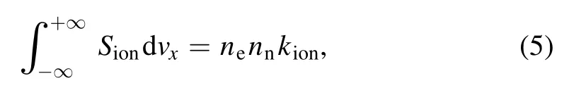
wherenerepresents the number density of electron andkionstands for the reaction rate coefficient given as a function of the electron temperature[1].The distribution ofSionin thevxdirection is assumed to be similar to that offn.Therefore,equation(5)is simplified as

2.2.Electron fluid model
The quasi-neutrality assumption is assumed in the hybrid model[19].The Debye length of the bulk discharge plasma in HTs is typically 10 μm,which is much smaller than the 10 mm discharge channel length.Consequently,the effects of charge separation are neglected for simulating the bulk plasma.The relationne=niis used.
The 1D electron fluid model consists of the conservation equations of mass,momentum,and energy.With the quasineutrality assumption,the mass conservation is written in the form of the equation of continuity as
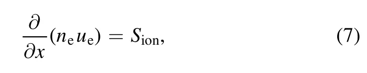
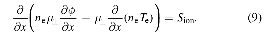
whereuerepresents the electron flow velocity.In the conservation equation of electron momentum,the electron inertia is neglected.The drift-diffusion equation is derived as

Therein,μ⊥represents the electron mobility across magnetic lines of force.The model for the cross-field electron mobility is explained later in this section.By substituting equation(8)into(7),an elliptic equation(diffusion equation)is obtained as
In the energy conservation equation,the kinetic component is ignored.The equation is written in terms of the electron internal energy as
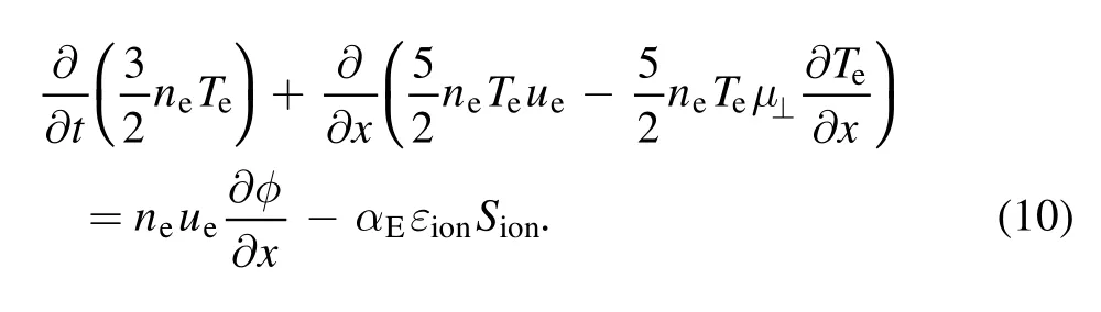
The second and third terms on the left-hand side respectively denote the enthalpy convection and heat conduction.The first and second terms of the right-hand side are the Joule heating and energy losses by inelastic collisions.The coefficientαEis a function of electron temperature determined for xenon,which is used conveniently to include energy losses by ionization,excitation,and radiation[1].Also,εionrepresents the ionization potential of xenon.
The cross-field electron mobility is modelled using a combination of classical diffusion and anomalous components as
whereμ⊥,claandμ⊥,anorespectively denote the classical and anomalous electron mobilities.The classical electron mobility is written as
whereμestands for the mobility of non-magnetized electrons asμe=e/mevela.The anomalous electron mobility is modelled by a Bohm-type diffusion model as

whereαBis designated as the Bohm diffusion coefficient herein.
The Bohm diffusion coefficient αBis given empirically as a function of the axial position.Several models have been proposed for the distribution ofαB[20].For this study,the three-region model[21]is adopted,whereαB=0.14 near the anode,αB=0.02 around the channel exit,andαB=0.7 in the plume region.These values are interpolated using the Gaussian functions[5]to obtain a smooth axial distribution ofα.B
2.3.Numerical method
2.3.1.Strang splitting.The nonlinear Vlasov equation with
ionization source term in equation(3)can be split into a series of linear partial differential equations through Strang splitting[22].The following steps are performed in one time loop:
(1)Solve the ionization ?tf-Sion=0with time step Δt.
(2)Calculate ?tf+vx?xf=0with time step Δt/2.
(3)Update the electric field and electron temperature through the fluid model.
(4)Calculate ?tf+eEx/mi?tf=0with time step Δt.
(5)Repeat step 1.
2.3.2.CIP-CSL scheme.This study used the SL method to solve the linear advection equations which are presented in the preceding subsection.To maintain the mass conservation and balance the flux between each grid,the CIP-CSL approach is used[23].The SL method is a grid-based approach.Therefore,it includes numerical diffusion in the velocity distribution.A fourth-order WENO limiter is incorporated with the CIP-CSL method to achieve high resolution in the velocity distributionwhile maintaining the small numerical oscillation.Additionally,the CIP-CSL method is known to compute the phase speed of high-wavenumber components accurately in wave propagation analysis[24].This property is anticipated as especially beneficial for plasma oscillation analysis.
2.3.3.Numerical method for electron fluid.The space potentialφand electron temperatureTeare obtained through the electron fluid model.The diffusion equation in equation(9)is solved for.φThe diffusion terms forφand pressure are discretized using central differencing.A direct matrix-inversion method is used to obtain theφdistribution from the discretized equation set.The energy conservation equation in equation(10)is used to deriveTe.The convection term of enthalpy folw is discretized using a second-order upwind method.A minmodtype flux limiter is used to gain the stability of the calculation.The diffusion term of heat conduction is discretized by secondorder central differencing.The second-order differencing methods are used in the electron fluid model because the distributions of the plasma parameters such asne,Te,andφ,are smooth in thex-(axial-)direction in HTs.Equation(10)is treated as a time-dependent equation.Time integration is implemented using a fully implicit method.
Equations(9)and(10)are calculated iteratively to obtainφandTe.The time step for the electron fluid is set to one-tenth of the time step for ions and neutral particles,i.e.ten electron sub-loops are used in a single time step for heavy particles.The electron mobility is calculated only in the first electron sub-loop.The computational grid in the 1D space for the electron fluid is the same as that for the Vlasov equation solver for ions and neutral particles.
3.Verification of the Vlasov solver
3.1.1D scalar wave propagation problems
The 1D scalar wave propagation problems are solved to verify the designed order of accuracy in the Vlasov equation solver.The SL method includes a series of advection-equation calculations.Each calculation can be checked through a scalar advection problem.Sinusoidal and square wave propagation problems with periodic boundary conditions are selected as test cases.In the sinusoidal wave propagation problem,the order of space accuracy is checked by comparing the numerical results with the analytic solution.The time step is set to be sufficiently small so that the discretization error deriving from the time-derivative term is negligibly small.Table 1 presents results of error analysis for this problem.TheL2norm of error decreases asO(Δx4).The fourth-order of accuracy designed by the WENO limiter is confirmed.The square wave propagation problem is solved to examine unexpected overshooting or undershooting.Figure 1 presents results of the square wave propagation problem obtained using the Vlasov equation solver with the fourth order WENO scheme and second order scheme.For the WENO limiter result,the original square waveform is maintained well.No overshooting or undershooting is observed in the result.As a reference,the same problem is solved with the total variation bounded(TVB)type limiter[17].Results obtained with the TVB limiter indicate that the waveform is distorted by the numerical diffusion near discontinuities.Test problems of the scalar advection problem confirmed that the developed Vlasov equation solver produces non-oscillatory results with a high order of accuracy.
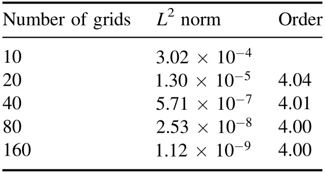
Table 1.Order of accuracy for 1D sinusoidal wave propagation.
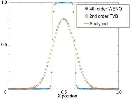
Figure 1.Numerical results of 1D square wave propagation with fourth order WENO and second order TVB limiters.

Table 2.Parameters for thruster operation assumed in the simulation.
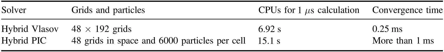
Table 3.Vlasov solver and hybrid PIC solver convergence speeds.
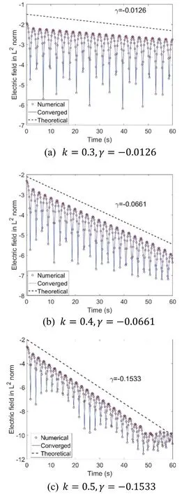
Figure 2.Time history of electric field in L2 norm,with wavenumber of(a) k=0.3,(b) k=0.4,and(c) k=0.5.
3.2.Vlasov-Poisson(VP) system
In this subsection,the CIP-CSL with a fourth-order WENO limiter is applied to the Vlasov equation in the VP system.The periodic boundary conditions are applied in the space direction.Impermeable wall boundary conditions are applied in the velocity direction.The 1D Poisson equation is solved through a direct integral method.The VP equation system is presented below.
here the sign of electric field in equation(15)is negative because the electron is handled in the VP system[25],whereas the ion number density is assumed to be uniform.Because this system handles only electrons,the model is not equivalent to a full PIC model nor a hybrid PIC model.However,this system has been conveniently used for the verification of Vlasov equation solvers for plasma simulations.The calculation domain is0≤x≤π/kand- 2π≤vx≤2π.The grid number reads 48 points in thexdirection and 100 points in thevxdirection.
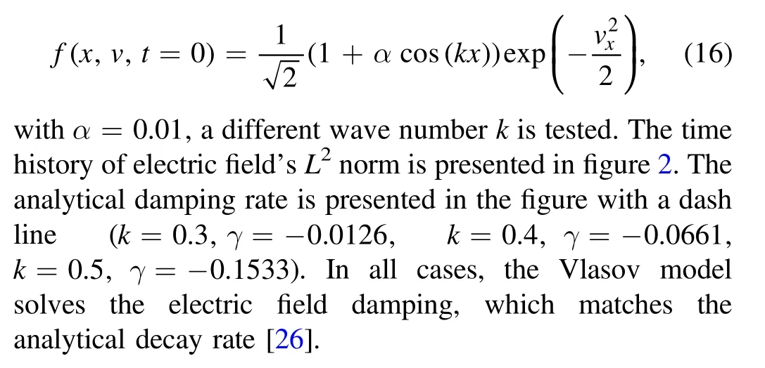
3.2.1.Weak Landau damping.The initial condition of weak Landau damping for VP system is
3.2.2.Two stream instability.To investigate how the noise is reduced by the Vlasov equation solver,the two-stream instability problem is simulated.The initial condition reads:
whereα=0.05,k=0.5.
For comparison,the same test case is also solved using the PIC[18]model,and the electric field is solved through the Poisson solver based on the central scheme.The equation of motion for each macroparticle is computed using a secondorder leap-frog method.A piecewise linear function is used for weighting between the particle positions and grid points.The number of grids in thex-direction is 48.The average number of macroparticles per cell is 100.The computational costs are almost equal between the Vlasov equation and particle solvers when they are solved using sequential computations.Figure 3 presents numerical results of the two-stream instability problem.The basic characteristics of distribution function for both models exhibit the same tendency.However,the result calculated using the PIC model includes much statistical noise,whereas the Vlasov equation solver achieves a noiseless result without overshooting or undershooting.The benefits of noiseless distribution of the Vlasov equation solver are confirmed.
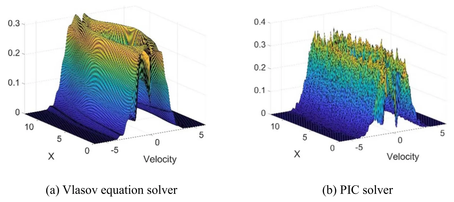
Figure 3.Numerical results of temporal distribution functions obtained using the(a)Vlasov equation solver and(b)PIC solver at t=30 s.

Figure 4.Flowchart of the hybrid Vlasov-fluid solver for HTs simulation.
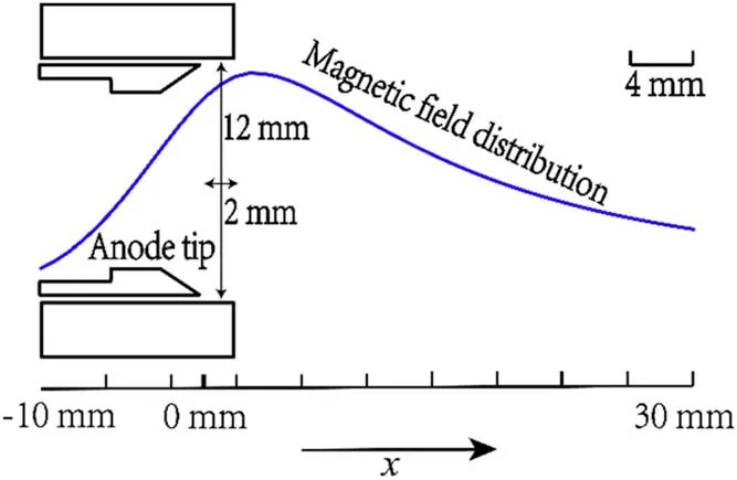
Figure 5.Axial-radial schematic of the Hall thruster considered in the present 1D simulation.The 1D calculation domain and magnetic field distribution are presented.
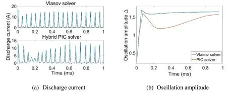
Figure 6.Time histories of the(a)discharge current and(b)oscillation amplitude with the classical diffusion coefficient.
4.1D1V simulation of ionization oscillation in HT
The simulations are running on a 2.9 GHz CPU with 32 GB memory,the hybrid Vlasov solver spends 1.92 h to finish the 1 ms simulation,meanwhile the hybrid PIC solver which employs 6000 macroparticles per cell takes 4.20 h.The calculation process of the hybrid Vlasov-fluid solver is demonstrated in figure 4,the calculation domain and initial distribution function are assumed as the input process.In the beginning,new ions are generated through the ionization process and added to the ion distribution function.The same number of particles is eliminated in the neutral distribution function.Then,ions and neutrals are advected by the Vlasov equation solver for half physical time step in space.Notice that neutral particles only have a single velocity,it does not propagate in the velocity space.Then the ion and neutral number densities are generated by integrating ion and neutral’s distribution function.These parameters are transferred into the electron fluid solver to calculate space potentialφand electron temperatureTeiteratively.Onceφis updated,the electric field is updated.Finally,the ions and neutrals are propagated for a fully physical time step invdirection and another half physical time step inxdirection.The hybrid PIC solver used in this study is the same as Dr Kawashima presented in[18],and this is the reduced one-dimension version of the two-dimensional model.The equation of motion for each macroparticle is computed using a second-order leapfrog method.A piecewise linear function is used for weighting between the particle positions and grid points.
4.1.Calculation conditions
The Vlasov equation solver is coupled with the magnetized electron fluid model for a HT simulation.The simulation target is the HT developed at The University of Tokyo[27].An axial 1D1V simulation is performed.The thruster operation parameters assumed for the simulation are presented in table 2.An axial distribution of magnetic flux density is assumed based on the measured data.The schematic of the HT calculation domain and the magnetic field distribution are portrayed in figure 5.The calculation domain contains the anode,discharge channel,and plume regions.The left-hand and right-hand side boundaries respectively correspond to the anode and cathode.The hollow anode model used in this study is the same as[28].To reflect the effect of the hollow anode in the simulation,the artificial electron mobility is employed in the region inside the hollow anode(-10 mm<x<0 mm).That is,the collision frequency inside the hollow anode is changed formvcolto(1+αHA)vcol.Here,the hollow anode parameterαHA=1is used.
After the propellant gas of xenon is injected into the domain from the left-hand side,it is ionized in the domain,and ejected from the right-hand side boundary.In the grid-based Vlasov equation solver,the minimum and maximum velocities are set respectively to-5 km s-1and 18 km s-1.192 grids are used in the velocity domain;48 grids are used in the space domain.The time step is set to 1 ns to satisfy the CFL condition for the Vlasov equation solver.With this time step,the CFL numbers are calculated as.
4.2.Boundary conditions
For the inlet and outlet boundary condition,the particles that flow into the calculation domain withu>0 atx=0 andu<0 atx=L,wherex=0 is the left-end andx=Lis right-end of the calculation domain.If the shape of the distribution function is smooth,simply Lagrange polynomial with the same order of the scheme can be used for the extrapolation to keep the same resolution at the boundary.
The boundary condition invdirection is simply to implement if the upper boundary and lower boundary are large enough.The distribution function at the boundary will become zero since there are no particles near each velocity boundary.The Dirichlet boundary condition can be set as zero in the ghost cell and Neumann condition can also be set as the gradient equal to zero.
The boundary conditions for space potential φ and electron temperatureTeare set for calculating the electron fluid.The Dirichlet condition of φ=250 V is used at the lefthand side boundary atx=-10 mm to apply the discharge voltage,and φ=10 V is assumed at the right-hand side as the beam plasma potential.Teis assumed to be 3 eV at the right-hand side boundary,and the Neumann condition of?Te/?x=0 is used at the left-hand side to make the heat conduction flux zero on the anode.
One of the features of the thruster with anode layer used in the present study is the hollow anode.The hollow anode model used in this study is the same as[28].To reflect the effect of the hollow anode in the simulation,the artificial electron mobility is employed in the region inside the hollow anode(-10 mm<x<0 mm).That is,the collision frequency inside the hollow anode is changed formvcolto(1+αHA)vcol.Here,the hollow anode parameterαHA=1 is used.
4.3.Comparison of computed results by Vlasov solver and conventional PIC Solver
During HT operation,ionization oscillations at frequencies of several tens of kilohertz are often observed.They have been investigated using several numerical models[29-32].This study examines the reproducibility of the characteristics of ionization oscillation using the developed Vlasov-fluid model.As a reference,a hybrid particle-fluid[18]simulation has also been performed.The obtained characteristics of ionization oscillation are compared between the hybrid Vlasov-fluid and hybrid PIC-fluid models.
4.3.1.Ionization oscillation.The oscillation amplitude Δ of discharge current is used as a criterion for the ionization oscillation.

In that equation,Idrepresents the time-averaged discharge current,Id,istands for the time varying discharge current,andNdenotes the number of samples.
Figure 6 presents discharge current oscillation and oscillation amplitudes over time for the case in whichBr,max=16 mT with classical diffusion.Here,anomalous electron mobility is not used.The calculation grids for the Vlasov solver are 48 grids in space and 192 grids in velocity.The hybrid PIC solver is calculated on the domain of 48 grids.The number of macroparticles is 6000 per cell,which is the minimum macroparticle number for a converged calculation.The Vlasov solver achieved a quasi-steady state oscillation mode with constant oscillation amplitude in a very short time.However,in results obtained from a hybrid PIC simulation,the oscillation amplitude is not stable because of the static noise.It is difficult to judge if the simulation reaches a quasisteady state of coherent waveforms.This unstable oscillation amplitude continues for a long time even if the simulation is performed as exceeding 1 ms.The Vlasov solver generated a steady oscillation waveform within the 1 ms simulation.The convergence speed for the steady oscillation amplitude is presented in table 3.In addition to the slow convergence speed,the computational cost(CPU seconds)for a given period of simulation is large when using the hybrid PIC method.This high cost is attributable to the large macroparticle number used for the simulation.In fact,the number of macroparticles in the simulation domain is less than 100 during lowId,although the average macroparticle number is approximately 6000.During lowId,most of the ions are exhausted.Neutral particles are depleted.Consequently,the number of particles in the hybrid PIC method cannot be decreased.The computational cost becomes large.
Here the macroscope plasma properties are calculated by taking the velocity moments of the VDF:
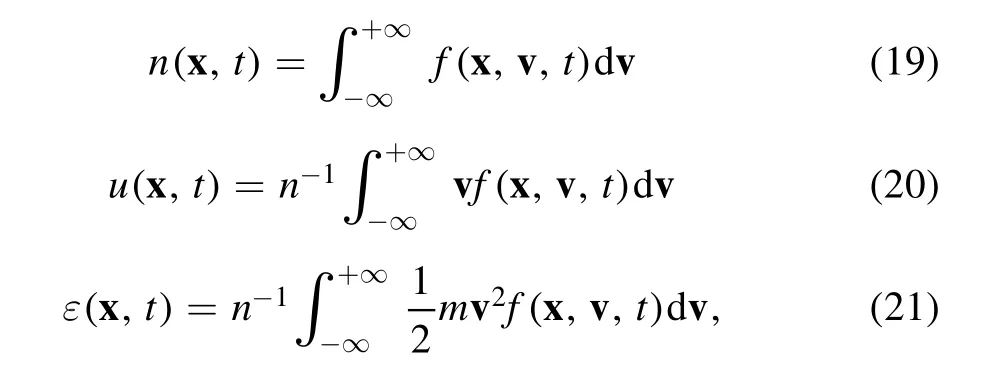
wherenis the number density,uis the mean velocity andεis the mean energy.As quasi neutral assumption is employed,the space potentialφand electron temperatureTeare calculated from the electron solver.
Figure 7 presents the time-averaged plasma properties of the solvers.The plasma properties generated by the hybrid Vlasov-fluid solver(square marker)show a similar distribution as the hybrid PIC solver(star marker).The space potential and electron temperature distribution show a good agreement between the two solvers,which guaranteed the similar mean velocities in each cell,these parameters may affect the total performance of HTs.The hybrid Vlasov-fluid solver also calculates the accelerate region correctly in comparison with the hybrid PIC solver.The plasma behaviours during the ionization oscillation are fundamentally the same for the two solvers.

Figure 7.Time-averaged plasma properties,left:neutral and ion number density,right:space potential and electron temperature,calculated with classical diffusion coefficient, Br, max=16 mT.Square:hybrid Vlasov-fluid solver,Star:hybrid PIC solver.

Figure 8.Simulation results of discharge oscillation amplitude.
4.3.2.Oscillation amplitude.Figure 8 presents discharge oscillation amplitude changes with different peak magnetic flux densities.Both the hybrid Vlasov-fluid solver and hybrid PIC solver show a trend that is similar to that observed in the experiment[33],although the PIC solver simulation collapsed when the maximum magnetic flux density was less than 15 mT in the classical diffusion case and 12 mT in the Bohm diffusion case because,when hybrid PIC solver runs in the low magnetic flux density region,the neutral number density becomes extremely small at the peak discharge current timing,resulting in divergence of the electron fluid solver.In this case,the hybrid PIC solver is unable to generate reasonable results with this number of macroparticles.By contrast,the Vlasov solver shows stable reproducibility in a wide magnetic flux density range,even with the same computational cost.
This work is the first step of hybrid Vlasov-fluid solver for Hall thruster simulation.We plan to go on with the 2D2V simulation to study the azimuthal rotating spoke and electron drift instability in the future.
5.Conclusions
In this study,we developed a hybrid Vlasov-fluid model for the ionized plasma flow.By replacing the particle solver for heavy particles with a SL Vlasov solver,a noiseless result was achieved with rapid convergence speed.For the Vlasov equation solver,the CIP-CSL method with fourth-order WENO limiter is employed to achieve high spatial resolution and non-oscillatory simulation.The fourth-order accuracy in space and non-oscillatory properties was verified using 1D scalar test problems.Test case of the VP system was used to verify the Vlasov solver.The noiseless feature was demonstrated with two-stream instability.A 1D1V simulation was performed for ionization oscillation analysis of HT.The trend of oscillation amplitude along with the magnetic flux density reproduces the trends observed in experiments.The noiseless Vlasov-fluid model yields quasisteady oscillation mode with a constant amplitude within a short simulation time compared with the hybrid PIC model.Furthermore,the Vlasov-fluid model shows a wider calculation range than that of the hybrid PIC solver in the low magnetic flux density region.The proposed SL Vlasov solver presents the benefit of resolving short wavelength oscillation.It is expected to be applicable to multi-dimensional simulations such as sheath problems and plasma drift instability problems.
Acknowledgments
This work was supported by the China Scholarship Council(No.201708050185).
 Plasma Science and Technology2022年2期
- Plasma Science and Technology的其它文章
- Investigation of short-channel design on performance optimization effect of Hall thruster with large height-radius ratio
- Multi-layer structure formation of relativistic electron beams in plasmas
- Mode structure symmetry breaking of reversed shear Alfvén eigenmodes and its impact on the generation of parallel velocity asymmetries in energetic particle distribution
- Interaction between energetic-ions and internal kink modes in a weak shear tokamak plasma
- Investigation of the compact torus plasma motion in the KTX-CTI device based on circuit analyses
- Anomalous transport driven by ion temperature gradient instability in an anisotropic deuterium-tritium plasma