
Passive robust control for uncertain Hamiltonian systems by using operator theory
2022-12-31 03:44NiBuYuyiZhangXiaoyongLiWeiChenChanganJiang
Ni Bu|Yuyi Zhang|Xiaoyong Li|Wei Chen|Changan Jiang
1College of Automation and Electronic Engineering,Qingdao University of Science and Technology,Qingdao,China
2Department of Robotics,Osaka Institute of Technology,Osaka,Japan
Abstract In this study,the passivity‐based robust control and tracking for Hamiltonian systems with unknown perturbations by using the operator‐based robust right coprime factorisation method is concerned.For the system with unknown perturbations,a design scheme is proposed to guarantee the uncertain non‐linear systems to be robustly stable while the equivalent non‐linear systems is passive,meanwhile the asymptotic tracking property of the plant output is discussed.Moreover,the design scheme can be also used into the general Hamiltonian systems while the simulation is used to further demonstrate the effectiveness of the proposed method.
KEYWORDS Hamiltonian systems,robust right coprime factorisation,storage function
1|INTRODUCTION
The Hamiltonian system has a prominent symmetrical form,and the Hamiltonian function itself is an energy function,with the most obvious regularity of motion;meanwhile,compared with Newton System and Lagrange System,the Hamiltonian system are most applied into the real applications[1,2],that is,all conserved real physical processes can be expressed in the Hamiltonian form,whether classical[3,4],quantum[5,6]or relativistic,whether the number of degrees of freedom is finite[7]or infinite[8,9],as is well known that the Hamiltonian function is one form of energy function;meanwhile,another method—passivity‐based control method is also based on the change of the energy and by redistributing the energy to achieve a satisfactory control performance.The passivity‐based control method(PBC)proposed in refs.[10–12]is based on the change of system energy and redistributes the energy to achieve a satisfactory control performance.Passivity‐based control method is different from the traditional control methods which are based on the feedback error signal.It fully reflects and utilises the physical structure characteristics of the system,that is,according to the specific characteristics of the system,an appropriate energy storage function is constructed to guarantee the passivity of the Hamiltonian systems[13–15].
Non‐linearity and uncertainty exist in most of the real dynamics in which the energy exchanges[16–18],therefore it is of great significance on studying the robust passive control for the uncertain non‐linear systems(UNS),especially for the UNS in the form of Hamiltonian system.Firstly,the passive systems take an important part in internal energy exchanging with outside.In detail,the energy stored in the passive system cannot be more than supplied one,while the difference is the dissipated energy.Different from the description by using the state‐space,the passivity is independent from the state by only considering the exchanges of the energy which simplifying the design and control for the dynamical systems and given this property,the PBC has been a hot topic by an increasing number of researchers.Secondly,non‐linear dynamics accounts for most of the controlled systems in system engineering,where the mathematical model can not be obtained exactly since the uncertainties usually exist,for example,the disturbance,and sometimes the performance cannot be satisfied by only approximating the considered systems into linear mathematical models,therefore,the design and control is important and essential for the UNS,especially for the robust design and robust control schemes,a stabilising controller is usually found to stabilise the systems.Some methods are proposed,for example,the Lyapunov method,gain scheduling method,feedback linearisation method,while most of the above mentioned methods assume that it is available to measure all the states.However,it is less line with the real practice because not all the states can be measured owing to some economic or instrument accuracy issues,thus the operator‐based robust right coprime factorisation method(ORRCF)[19,20]is referred,which is a useful method in controlling and designing the UNS by which it is no need to consider the measurement of the states.
The ORRCF method is mainly concerned with the relationship between the input‐output mapping without the discussion of the measurement of the states,and the adopted extended linear space will be more suitable for the real applications.Furthermore,by establishing a Lipschitz norm inequality and the Bezout identity[20],the non‐linear feedback control systems(NFCS)will be robustly stable.In the following statements,the existing results by the endeavours as well as the unsolved problems will be simply introduced.
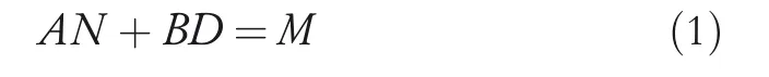
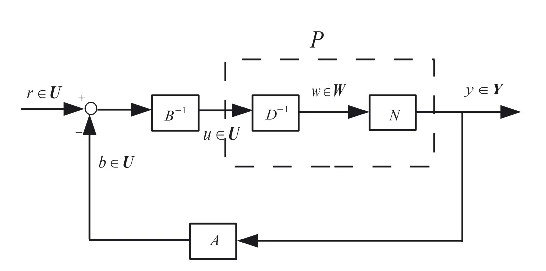
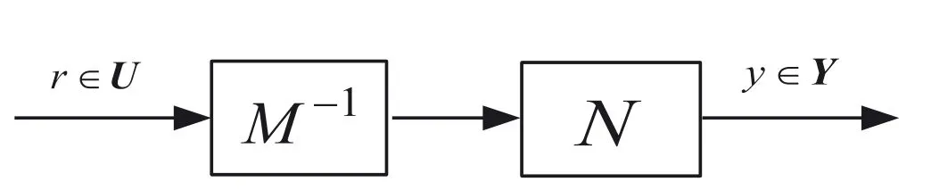
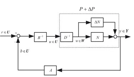
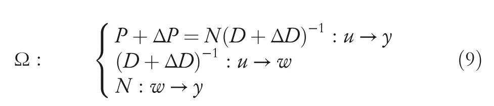
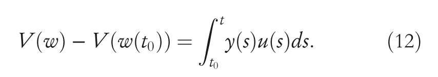
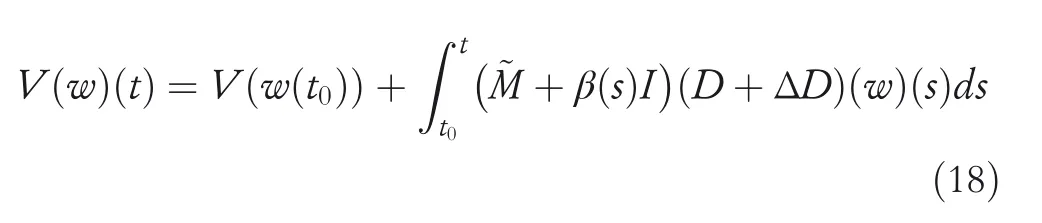
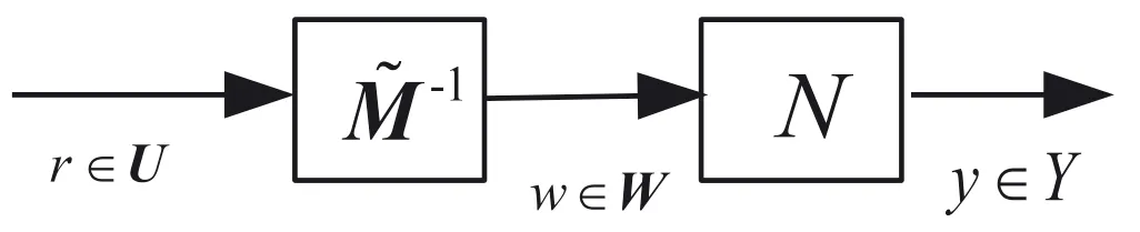
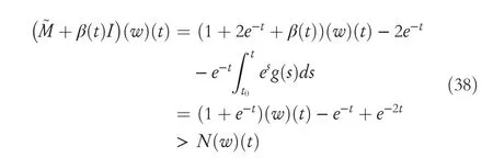
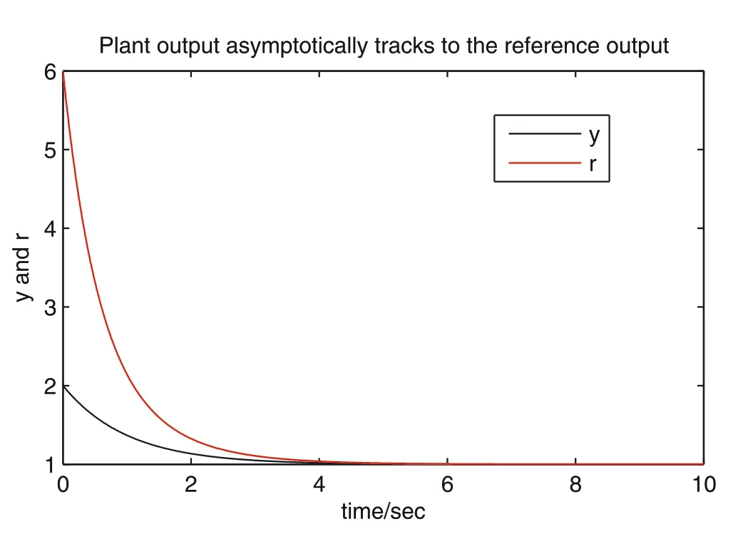
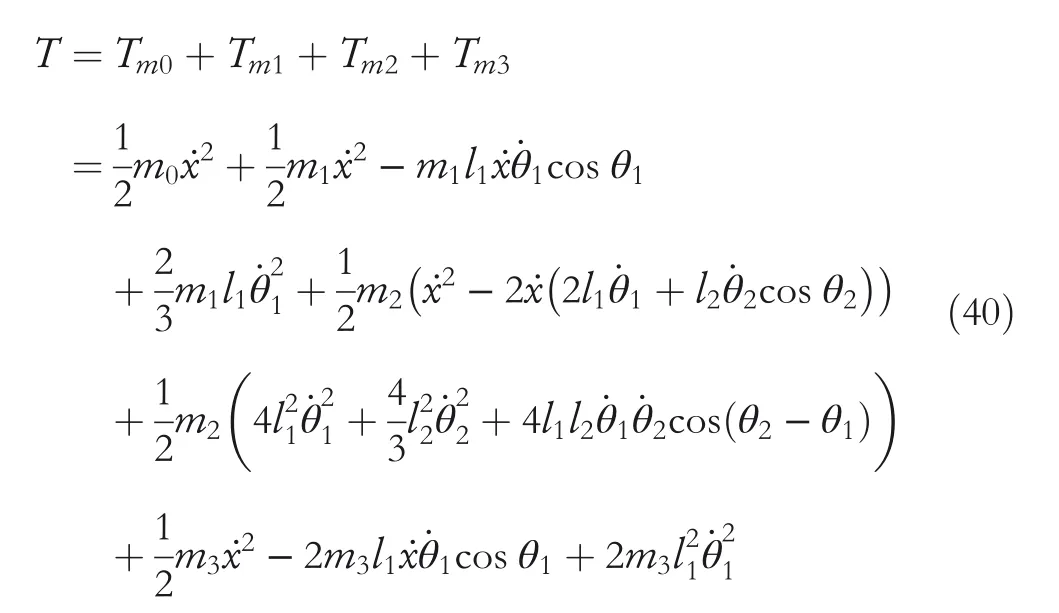
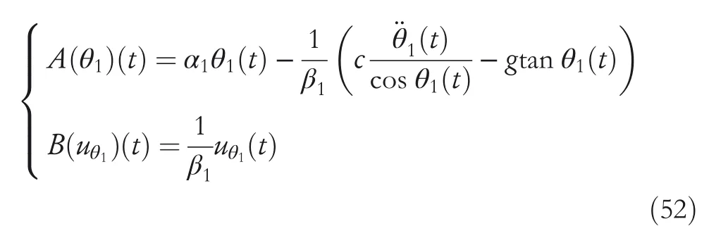
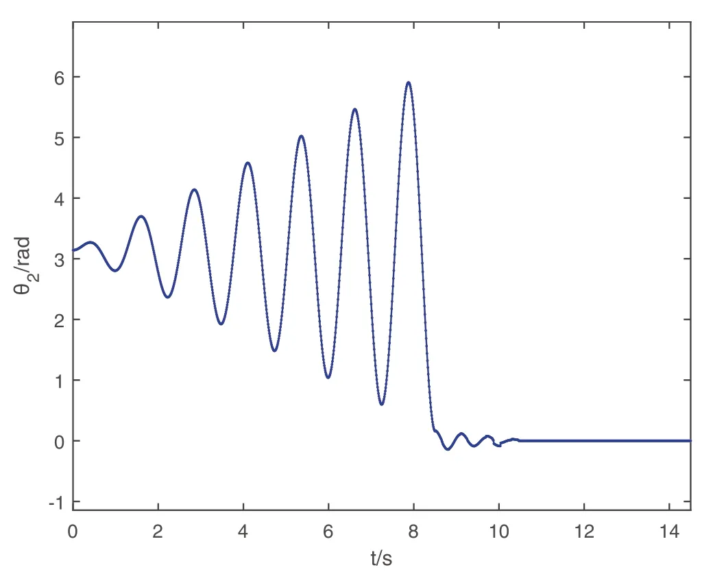
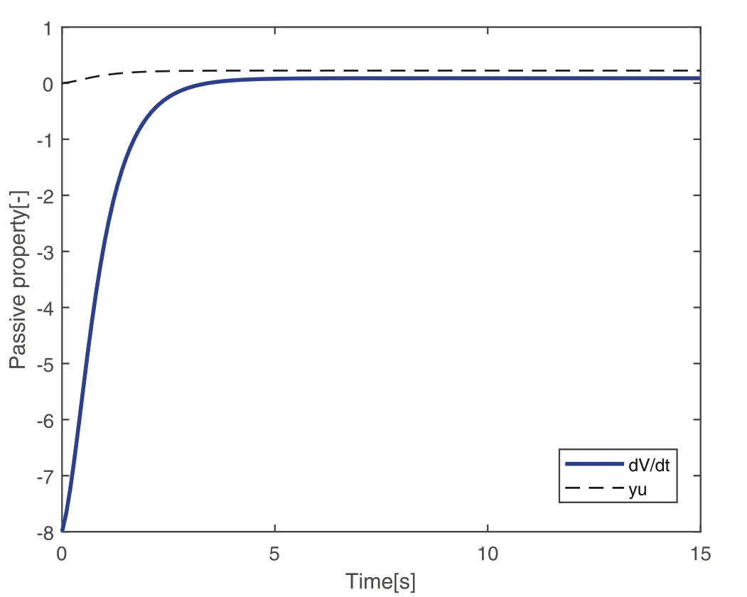
By the increasing requirement of the robust control for the non‐linear systems,where the uncertainties usually exist and cannot be completely offset which leads to the unsatisfactory performance,a wider inequality condition is proposed based on the Lipschitz norm proposed in ref.[20],which can be applied in the real systems and thus the method of ORRCF has been widely applied in more and more real systems[21–26].On the existing results of the ORRCF method,another fundamental issue is seldom discussed–the factorisation method,therefore on this topic,we considered it and realised the factorisation of the non‐linear plant in refs.[27,28],moreover,the combination of the PBC and ORRCF is also discussed[29,30];however,in this result,the robust controller is designedA?Iwhich is limited the applications while the storage function is designed in two cases~M≥Nand~M Therefore,the contributions of this paper are summarised:(1)The design scheme combining the operator‐based robust right coprime factorisation(RCF)and the PBC is extended into the design and control for the Hamiltonian system which is more popular in the modelling of the physical dynamics.(2)The general robust controller is designed which extends the application of the existing results,by which the asymptotic tracking performance can be improved while the robustness is maintained.(3)By introducing the adjustment variable,a general form of the storage function is constructed to ensure that the passivity of the uncertain non‐linear feedback system to overcome the disadvantage of two different storage function. The following is the framework of this paper:Section 2 includes the basic definitions about operator theory and the passivity properties.In Section 3,the main results are demonstrated,that is the ORRCF control PBC.In Section 4,the simulation will be provided,which further demonstrates the feasibility of the proposed design scheme.The final part describes the conclusions of the paper. 2.1.1|Operator theory Some definitions as well as existing results of operator theory will be introduced in this part. Here,operatorP:U→Y,whereU:input space,Y:output space,with their normed subspace is respectively denoted to beUsandYs,where?x1,x2∈U,thenUsandYsarestable subspaces. If the operatorP:D(P)→Yexists,where D(P)and R(P)is respectively the domain and the range.The following rule holds:P:α1u1+α2u2→α1P(u1)+α2P(u2)forui∈D(P)withαi∈C,(i=1,2),thenPcan be called to be linear operator.The operators that D(P)=U,R(P)?Ywill be discussed in this paper. Definition 2.1P:U→Yis Bounded Input Bounded Output(BIBO)stable,withP(Us)?Ys,it can be simplified to be BIBO stable. Define?(U,Y):Us→Ys,then?(Us,Ys)includesμ(Us,Ys)={M:M∈?(Us,Ys)which are denoted to beunimodular operators. Definition 2.2The operatorP:U→Ydescribes a system from the input spaceUinto the output spacesYwhich is in‐out stable.If the operator norm is finite,that is,‖P‖<∞,the system isfinite‐gain input‐output stable. The definitions about RCF will be introduced as follows: Definition 2.3DefineP=ND?1,then it iscoprime,if the Bezout identity is satisfied,whereAandBare the designed controllers with the unimodular operatorM.That is,NandD?1is said to be the RCF ofP. Note:the initial condition should also be met with:AN(w0,t0)+BD(w0,t0)=M(w0,t0). LetM∈[0,∞).ForT∈[0,∞)that is constant,andPT:M→MT,which are both linear spaces. wherefT(t)∈MT.Then, We can denote that,Xeis theextended linear spacecorresponding toXB,which is the notated Banach space. Definition 2.4LetDe?Ue,thenFis denoted to bea generalised Lipschitz operator(GLOP)withF:De→Yeand the following condition holds whereu,~u∈DeandT∈[0,∞).Lip(De)means the family of non‐linear GLOPs that mapDeto themselves.Lis obtained by 2.1.2|Robust right coprime factorisation Definition 2.5Considering?r∈U,the system iswell‐posed,if all the signals in Figure 1 are unique. Definition 2.6In Figure 1,ifr∈Us,e∈Us,u∈Us,w∈Ws,y∈Ysas well asb∈Us,then NFCS shown in Figure 1 can be saidoverall stable. FIGURE 1 The operator‐based NFCS. In ref.[19],the authors derived a useful result for the relationship between the stability of the NFCS shown in Figure 1 and RCF,that is,if Equation(1)is satisfied,then the NFCS is overall stable.Furthermore,because of the satisfaction of the Bezout identity,Figure 1 can be equivalent to Figure 2[19]. Moreover,the ORRCF has been discussed in ref.[19],that is the sufficient condition is obtained,which means the effects of the uncertainties is offset.However,it is difficult to realise this condition.According to Lipschitz norm,the robust conditions in the form of inequality is proposed for the UNS shown in Figure 3.Therefore,the sufficient condition is given in Lemma 1[20]. FIGURE 2 Equivalent one with the system in Figure 1. FIGURE 3 NFCS with unknown perturbations. FIGURE 4 An uncertain non‐linear feedback system. Lemma 1Let De?Ue,if(A(N+ΔN)?AN)M?1∈Lip(De),and where‖·‖is defined in Equation(5),then NFCS in Figure 3 is stable. Therefore,if the condition Equation(8)is satisfied,thenMcan be said to be a unimodular operator,which means that Equation(7)is a Bezout identity,thus according to the result in ref.[19],the UNS shown in Figure 3 is also stable.The UNS will has robust stability since Equation(6)is also satisfied.Moreover,ifP+ΔP=(N+ΔN)D?1has a robust RCF,then the UNS has robust stability.For ease of understanding,the conditions Equations(6)and(8)arerobust conditions.If Equation(7)can be directly described to be a Bezout identity without some complex computations of Lipschitz norm in Equation(8),then we will go to the simplified one to verify whether the UNS is robustly stable. In Figure 4,the system Ω: whereu∈Uis the control input,w∈Wis the quasi‐state whiley∈Yis the plant output. Definition 2.7 Ω isenergy balancedif a non‐negative function which is calledstorage function V:W→R+exists,such that for?u∈U,w0∈W,t≥t0, The system Ω can be said to bepassive,that is, Furthermore,all the supplied energy is stored,that is,δ(t)=0, then the system Ω can be described to belossless.Actually,in most of the non‐linear dynamical systems,δ(t)=0 cannot hold.In this paper,the passive cases which hinge on more fundamental and universal property for the non‐linear dynamical systems are mainly discussed. If non‐negative differential functionVexists,the passivity inequality Equation(11)can be redescribed as In Figure 4,NFCS with perturbed plant is studied,whereP+ΔP=N(D+ΔD)?1withP=ND?1is the real and nominal factorisation.The unstable operators areP,P+ΔPand(D+ΔD)?1,while the others are stable and bounded with linearN,that is,all the non‐linear parts are included inD?1and(D+ΔD)?1. This paper discusses three problems.Firstly,in ref.[29],the robust controller is designed under the assumption of‘The plant output can track to the reference input perfectly for the nominal plant’which is hard to be realised and limited real applications,thus we will design a general scheme for the robust controllers.Secondly,in ref.[29],two cases of storage functions is given which is not feasible for the real applications,we will give a general design scheme of the storage function,which is more line with the practice.Thirdly,the design scheme will be extended into the control and design of the Hamiltonian systems. This paper studies the passive robust control for the UNS.Based on the proposed conditions,the passive robust controllers are designed with the general storage function,that is,the corresponding Bezout identity and the passive conditions are both satisfied.Therefore,the UNS is robustly stable and passive. The following sufficient condition ensuring the perturbed non‐linear feedback systems to be robustly stable and improved tracking performance is the development of the robust control scheme in ref.[29],where the proposed two conditions areA?IandAN+BD=M=Nwhich limited the application of the design and control of the non‐linear systems. Theorem 3.1In Figure 4,assuming the non‐linear system is well‐posed,if the stable linear controller A is designed as follows: then the robust stability and tracking performance of UNS can be guaranteed. Proof:Firstly,the nominal non‐linear system is stable since Equation(14)is satisfied as a Bezout identity. Secondly,for the UNS,it is obtained that Thirdly,since Equation(16)holds,then the NFCS is redescribed as the one in Figure 5. according to Equations(15)and(17),→Nast→∞,therefore,y→r,that is the system has good tracking performance.This complete the proof. In ref.[29],we considered two design schemes of the storage functions,which is not simplified or economical,therefore,in this section,we will again discuss the chosen of the storage function and a general construct scheme will be proposed. Theorem 3.2In Figure 4,assuming that a NFCS is well‐posed,according to Theorem 3.1,the control scheme can be designed to ensure that whereβ(t)is the variable for adjustment,then the whole UNS can be ensured to be strictly passive. Proof:If the storage function is designed as the above form,then By adjusting the variableβ(t),the results are obtained,whether>Nor FIGURE 5 Equivalent one of the system in Figure 4. therefore,we find that which means that then the NFCS is passive by designing the robust controllers.This completes the proof. The contribution lies in that this condition gives a universal construct scheme for the storage functionV,which is more line with the practice than constructed ones in ref.[29]. In 1833,William Rowan Hamilton formulated Hamiltonian mechanics firstly,starting from Lagrangian mechanics and developed into one of the three basic representation forms in the classical mechanic systems(Newtonian mechanics,Lagrangian mechanics and Hamiltonian mechanics).The Hamiltonian mechanics describe not only the usual mechanical dynamics but a bigger family of physical systems,by which all the real physical processes can be expressed,including the structural biology,celestial mechanics,plasma mechanics,material mechanics and so on,therefore the investigation of the Hamiltonian system is very important and in this part we will consider its control and design issues by using the above proposed design and control schemes. First,we consider the following Hamiltonian systems which is described in the operator form, In detail, wherew,u,yis respectively the quasi‐state,the control input,and the plant output,H(w)is the energy function,J(w)implies the structure of the systems,R(w)denotes the system dissipation andg(w)is the general coefficient of the control input which can be specially chosen to beIbut it can not be equal to 0 since the unstable system cannot be controlled without the input.According to the definition of the operator,it can achieved that. Theorem 3.3Consider the Hamiltonian systems Σ,where the two factors N as well as D+ΔD is respectively obtained by Equations(24)and(25),in order to satisfy the following conditions,the controllers A*and B*is respectively designed.Hamiltonian systems Σ is robustly stable while the passivity holds for the existing unimodular operator~M(w). Proof: 2)According toTheorem 3.3,Equations(27)and(28),we can find that the passivity of the Hamiltonian system holds. 3)Based on the definition of BIBO stability as well as Equations(26)–(28),A*andB*is proved to exist,this complete the proof. By giving a numerical example,the effectiveness arising from the above proposition will be illustrated. Assuming the perturbed plantP+ΔP:U→Yis as follows: whereu∈U,g(t)is the additive uncertaintyg(t)→0 ast→∞.According to the isomorphism method[27],the plant with disturbance is factorised. and It is obtained that the unstable operators areP+ΔPand(D+ΔD)?1,and the BIBO stable operators areNandD+ΔD.Then,the two controllersAandBis respectively designed to be such that thus then we verify the condition Equation(15) The following is the further verification: therefore,the designed system has robustness as well as good tracking performance which is demonstrated in Figure 6. Next,the passivity of the UNS will be verified for two cases,wheret0=0,g(t)=e?2t. i)If the reference inputr1(t)=1+2e?t+3e?2t,then the quasi‐state can be obtainedw=1+e?tand(D+ΔD)(w)(t)=?2e?2t<0,then we can designβ(t)=?e?tand then the passive property can be ensured according to˙V ii)If the reference inputr2(t)=?3e?t?3e?2t,thenw=?2e?tand(D+ΔD)(w)(t)=e?2t>0,then we can designβ*(t)=?2e?tand FIGURE 6 Case ii):Plant output asymptotically tracks to the reference output. FIGURE 7 Case i):Passive non‐linear system. In this part,the robust passive for the double inverted pendulum(DIP)will be given to demonstrate the validity of the proposed method,that is,a self‐swing control scheme combining ORRCF method and PBC is proposed[29].The control scheme consists of three steps.(1)The switching control law is designed to swing the first‐stage pendulum into a vertical inverted position.(2)From the perspective of the energy,by using the PBC method,the first‐stage pendulum is controlled to be stable in the inverted position.(3)The control scheme of combining ORRCF method and PBC is used to stabilise the two pendulums in the inverted position simultaneously,by which the influence of external perturbation during the switching process can be weakened. The physical model of the DIP is shown in Figure 10,and Table 1 includes the specific parameters.According to the physical rule,the total energy(potential energy and kinetic energy)of the DIP are expressed as follows: FIGURE 8 Case i):Plant output asymptotically tracks to the reference output. FIGURE 9 Case ii):Passive non‐linear system. FIGURE 1 0 Physical model of double inverted pendulum(DIP). TABLE 1 Physical parameters and The above equations are modelled by the proposed Hamiltonian method,and the dynamic equation of the DIP is obtained. and Meanwhile,the acceleration control method is adopted Considering the real case of the limited rail,the following conditions should be satisfied:(1)|x|<0.35 m,(2)|u|=||<40 m/s2. 4.2.1|The swing of the first‐stage pendulum This part is mainly to swing the first‐stage pendulum to near the inverted position,while coordinating the pacing of the two pendulums.For the swing‐up control,the switching control lawu1is designed using the energy control method of the PBC method. The controller is designed as follows: whereβ1>0 is the parameter that needs to be designed.The switching method includes two situations:(i)When the swing angle isθ1∈(π/2,π)orθ1∈(?π,?π/2)and the pendulum swings clockwise,the control input is?β1;When it swings counter‐clockwise,it is switched toβ1.(ii)When the swing angle isθ1∈(?π/2,0)orθ1∈(0,π/2)and the pendulum swings clockwise,the control input isβ1;When it swings counter‐clockwise,it switches to?β1. 4.2.2|Robust control of first‐stage inverted pendulum According to proposed design scheme for the DIP,the first‐stage inverted pendulum dynamics can be controlled: whereθ1≠±π/2,that is,the pendulum is not controllable when the pendulum is in a horizontal position,c=0.15 and the gravitational acceleration isg=9.8 m/s2. As Figure 3 shows,the corresponding symbol of the first‐stage inverted pendulum control system is represented by{P,N,D,M,A,B}.Firstly,we use the isomorphism‐based ORRCF method to realise the factorisation of the operator modelled DIP system: According to the definition of RCF,the mathematical model of the first‐stage inverted pendulum system is factorised According to the physical rules,the storage functionVPwith the input variableωis designed: where|M(ω)(t)|is no larger than|N(ω)(t)|. The differential representation of the stored function(ω)(t),as the passive condition which represents as: In following part,we will verify the robustness and the passivity of the DIP by means of the robust condition and the passive condition. Firstly,AN+BD=Mcan be satisfied with the designed robust controllers as follows: where 0<α1≤1,β1>0 are the parameters to be designed,then the stability of DIP is ensured. Meanwhile,the following passive condition is ensured by the proposed design scheme, wherey1(t)uθ1(t)=ND(ω)(t).Therefore,it shows that the designed controller guarantees the passivity of the system. Therefore,the designed control scheme guarantees stability and passivity for DIP,wherein the control switching law of the first‐stage inverted pendulum can be designed: wheree1(|e1|≤δ)is the error of convergence to the desired angle in the first‐stage inverted pendulum control. When the second pendulum swings to the vicinity of the vertical inverted position,the control law is designed to be the switching law.During this stage,the control method of combining the above ORRCF method and PBC is used to deal with the robustness of DIP.The variables presented in control system is described in Table 1.Based on the Taylor series around the equilibrium point and linearisation method,where the corresponding parts are respectively represented by{Pi,Ni,Di,Mi,Ai,Bi,e3i}.Thus,the mathematical model of the DIP system can be further simplified: Similarly,the control law of the secondary inverted pendulum is designed as follows: whereβ3i=[β31β32]Tis the parameters to be designed.|e3i|≤δ(i=1,2)is the error that the pendulum rod 1 and the pendulum rod 2 converging to the desired angle in the swing control. In summary,the overall control scheme of the secondary inverted pendulum system is summarised as follows: The parameters are selected as follows?2=0.113 rad,σ=1.049 rad,and simulation are carried out corresponding to the above parameters. The detailed control process is as follows,(1)The pendulum rod 1 starts to swing from the vertical downward position(i.e.|θ1|=π),and swings to near the inverted position at 6s with the control inputu1.(2)Next,the controlleru2is switched to play part in the control of DIP.As the controlleru21works,the oscillation of the swing angleθ1converges to zero(i.e.|θ1|≤?1).Meanwhile,the pendulum rod 2 is swung up to coordinate the pace between the two pendulum rods.(i)When|θ2|>σ,theu22is designed for the second‐stage pendulum rod to achieve the desired height of the swing;(ii)When|θ2|≤σtheu22is designed by the energy method to avoid energy dissipation.Specially:ifu22is too large,the buffeting of the system will be serious,then the first pendulum will not be able to stabilise in the vertical position;ifu22is too small,the system will not be able to provide enough energy for the second pendulum.Therefore,the value ofu22cannot be too large or too small,so that the pendulum rod 1 can be vertically inverted and the pendulum rod 2 can be smoothly swung up.That is to say,the value ofu22limits the displacement of the car to a certain extent,which also satisfies the condition that the guide rail is limited.(3)Finally,when the angle of pendulum 2 is within a certain range(i.e.?2≤θ2≤σ),it switches to the controlleru3,whileθθ2gradually oscillates and converges to zero. The control input signal is shown in Figure 11.Figure 12 and Figure 13 show simulation curves of DIP.The results imply the proposed control scheme can successfully realise the self‐swing control and swing the two pendulum rods to the inverted position in a short time.Meanwhile,the passive performance is demonstrated in Figure 14 by which we can find that the passivity of the DIP is guaranteed. That is,it is clearly seen from the simulation that the ORRCF method combined with the PBC control scheme makes the two swing angles converge to zero within 10s during the entire control process.At the same time,the two pendulum rods are stably maintained in the vertical upward position.Therefore,the designed control scheme ensures the fast convergence speed,strong robustness and the passivity for DIP. FIGURE 1 1 Control input signal u. FIGURE 1 2 Response curve of pendulum 1 angle θ2. FIGURE 1 3 Response curve of pendulum 2 angle θ2. FIGURE 1 4 Passive control performance. In this paper,the passivity‐based robust control for uncertain Hamiltonian system is discussed by combining ORRCF method with the PBC method in this paper,in details,the contributions include:(i)the robustness for the UNS is guaranteed designing the robust controllers,meanwhile,the asymptotic tracking performance is improved.(ii)By the designed robust controllers,a universal passive condition is proposed,by which the passivity for the UNS can be ensured.(iii)The general Hamiltonian system is modelled to the operator‐based form using the isomorphism‐based RCF,wherein the new storage function is chosen and the passive condition holds for the general Hamiltonian system.Finally,the numerical example and the simulation in spirit of the robust passive control for DIP are respectively given,from which the validity of the proposed control schemes are confirmed. Next,the proposed control schemes will be applied into the Hamiltonian system with time delay and more general non‐linear feedback systems,for example,the hysteresis modelling soft micro‐hand.Meanwhile,the method will be improved to combine with sliding mode control and other intelligent methods to deal with the identification and the optimisation of the tracking control methods. ACKNOWLEDGEMENT This work was supported in part by the National Natural Science Foundation of China of No.61304093 and the Natural Science Foundation of Shandong Province of No.ZR2021MF047. CONFLICT OF INTEREST The author declares that there is no conflict of interest that could be perceived as prejudicing the impartiality of the research reported. DATA AVAILABILITY STATEMENT The data that support the findings of this study are available from the corresponding author upon reasonable request. ORCID Ni Buhttps://orcid.org/0000-0001-5046-1743 Changan Jianghttps://orcid.org/0000-0001-8105-78232|MATHEMATICAL PRELIMINARIES
2.1|Operator‐based robust right coprime factorisation


2.2|Passivity theory


2.3|Problem statement
3|MAIN RESULTS
3.1|Robust control scheme


3.2|Verification of passivity


3.3|Hamiltonian system design scheme


4|SIMULATIONS
4.1|Numerical example


4.2|Robust passive control for double inverted pendulum


5|CONCLUSION
 CAAI Transactions on Intelligence Technology2022年4期