
A Diffusive Predator-Prey Model with Spatially Heterogeneous Carrying Capacity
2023-02-15 06:40CHENJiaweiandWANGBiao
CHEN Jiawei and WANG Biao
College of Science,Xi’an University of Science and Technology,Xi’an 710054,China.
Abstract. We study local dynamics of a diffusive predator-prey model in a spatially heterogeneous environment,where intrinsic growth rate of the prey is spatially homogeneous,whereas carrying capacity of the habitat is spatially inhomogeneous.In comparison with the existing predator-prey models,the stability of semi-trivial steady state of this model displays distinct properties.For example,for certain intermediate ranges of the death rate of the predator,the semi-trivial steady state can change its stability at least once as the dispersal rate of the prey varies from small to large,while the stability of the semi-trivial steady state is immune from the dispersal rate of the predator.
Key Words: Predator-prey model;carrying capacity;spatial heterogeneity;stability.
1 Introduction
The movement of organisms is often crucial to its persistence.The creatures are scattered to look for resources,seek breeding habitat,and avoid predation,etc.Understanding the impact of dispersal on population dynamics is still an important topic in ecology.One way to investigate how the joint action of dispersal and spatial heterogeneity influences populations and communities is by using reaction-diffusion models [1].For instance,it was shown in[2]that for a reaction-diffusion model with logistic growth term in spatially heterogeneous environments,as long as a species keeps moving randomly,the total amount of resources always supports a population strictly larger than the total carrying capacity.Recently,this model has been generalized to be a more realistic one[3],where both intrinsic growth rate and carrying capacity depend on spatial variable in the habitat.Their outcomes indicate that the total population of the species has more complicated relations with the total carrying capacity.However,when the intrinsic growth rate is constant,while the carrying capacity is spatially heterogeneous,a striking result from[4]implies that for any diffusion rate,the total amount of resources supports a population strictly smaller than the total carrying capacity.For more research concerning the effects of diffusion rate and spatial heterogeneity of the environment on dynamics of populations via reaction-diffusion models,we refer interested readers to [5-13] and reference therein.
In this paper,we discuss a diffusive predator-prey model with spatially homogeneous intrinsic growth rate of the prey and spatially inhomogeneous carrying capacity of the habitat,and explore the effects of dispersal and spatial heterogeneity on the local dynamics of the predator and prey populations.The mathematical model can be characterized by the following reaction-diffusion system:
whereu(x,t)andv(x,t)represent the population density of prey and predator species at locationxand timetwith corresponding diffusion ratesμandν.The initial valuesu0(x)andv0(x)are both non-negative and non-trivial.The functionK(x)denotes carrying capacity of the habitat,andd>0 is the mortality rate of the predator.is the Laplace operator in RN,which characterizes the random movement of the predator and the prey species.The habitat Ω is a bounded domain in RNwith smooth boundary?Ω.The zero Neumann boundary conditions mean that no individual can cross the boundary of the habitat.?u/?n=?u·n,wherenis the outward unit normal vector on?Ω.The constantsμ,νandkare supposed to be positive.
To reflect spatial heterogeneity of carrying capacity of the habitat in (1.1),throughout this paper,we always assume that the carrying capacityK(x)satisfies the following condition:
IfK(x)satisfies(1.2),then the single species equation[3,4]admits a unique positive solution for everyμ>0,denoted asθ(x,μ),andθ(x,μ)∈C2().For the sake of simplicity,we frequently writeθ(x,μ)asθ.Therefore,under the assumption(1.2),the model(1.1)has a unique semi-trivial steady state(θ,0).
The purpose of this paper is to investigate local stability of the semi-trivial steady state(θ,0),it turns out that its stability is determined by the sign of the principal eigenvalue of an eigenvalue problem (2.12) with indefinite weights.Clearly,the principal eigenvalueλ1of(2.12)is a function of the dispersal rates of the predator and prey.Hence,it suffices to inquire about howλ1changes its sign as the dispersal rates of the predator and prey vary from small to large.To more precisely state the main results of this paper,we define some notations:
The magnitude ofd1,d2andd3can be obtained from Lemma 2.2 in Section 2,which is given byd1<d2<d3.
The main consequence of this paper is as follows:
Theorem 1.1.Suppose that(1.2)holds.Then the following conclusions are true.
(i)If d<d1,then(θ,0)is unstable for anyμ>0and ν>0.
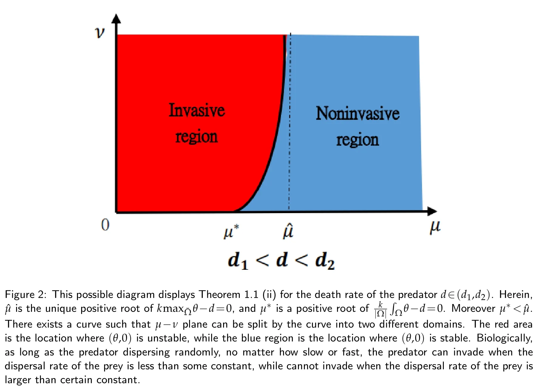
(ii)If d1<d<d2,and K(x)also satisfies(2.7),then for every ν>0,(θ,0)changes its stability at least once asμvaries from0to+∞.
(iii)If d2<d<d3,and K(x)also satisfies(2.7),then there exists a unique=(d,K,Ω)>0such that for any ν>,(θ,0)is stable for everyμ>0;whereas for any ν<,(θ,0)changes its stability at least once asμvaries from0to+∞.
(iv)If d>d3,then(θ,0)is stable for everyμ>0and ν>0.
Remark 1.1.If the carrying capacity of the habitat is a positive constant,thend1=d2=d3>0.The results of Theorem 1.1 reduces to (i) and (ii).In sharp contrast to spatially homogeneous carrying capacity,Theorem 1.1 reveals the process how the stability of(θ,0) changes from unstable to stable stepwise as the death rate of the predator varies from small to large,but not just simple from unstable to stable.

Figure 1: This picture illustrates Theorem 1.1 (i) for the parameter range d∈(0,d1).The red region is a place where(θ,0) is unstable,that is,the predator can invade when the predator is relatively rare.From the biological point of view,it implies that as long as the death rate of the predator is less than some constant,the predator will successfully invade when scarce,which is independent of the dispersal rates of the predator and prey.
Remark 1.2.The case when intrinsic growth rate of the prey is spatially heterogeneous and carrying capacity of the habitat is spatially homogeneous has been considered in[14].To compare the outcomes of Theorem 1.1 with that of[14,Theorem 1.1],we assume thatK(x)=m(x),wherem(x) is the intrinsic growth rate of the prey in [14].Part (iv) is the similar to [14,Theorem 1.1 (i)].However,asθhas opposite property with that of[14,Theorem 1.1],Parts(ii)and(iii)exhibit tremendous differences.Though the result of Part(i)is similar to that of[14,Theorem 1.1(iv)],the critical death rate of the predator is less than that of [14,Theorem 1.1 (iv)].Biologically,the predator with smaller death rate can invade when rare,which is independent of the dispersal rates of the predator and prey.
We shall apply the following four figures to explain the outcomes of Theorem 1.1.Figs.2 and 3 are drawn for illustrative purposes only,because the real curves separating the invasive and non-invasive regions should be more complicated.
The rest of this paper is arranged as follows: In Section 2,we give some qualitative properties ofθ,and establish a criteria for the stability of(θ,0).Section 3 is devoted to the proof of Theorem 1.1.In Section 4,we present some discussions for further investigation.
2 Preliminary
In this section,we firstly introduce several consequences ofθ,and then give a criteria for the local stability of(θ,0)and related properties.
Lemma 2.1.Suppose that K(x)satisfies(1.2).Then
(i)(x,μ)is a smooth mapping fromR+to C2().In addition,
uniformly on.
(ii)For every μ>0,<K andθ >K.In particular,‖θ‖L∞(Ω)<‖K‖L∞(Ω).
Proof.The smooth dependence ofθonμcan be obtained from the implicit function theorem[1].The limiting behaviors ofθasμapproaches zero or infinity can be found in[3].Part(ii)can be derived by the maximum principle(see,e.g.,[15]).
Lemma 2.2.For everyμ>0,we have
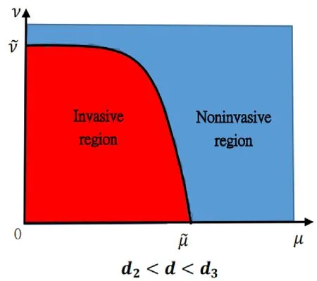
Figure 3: This possible figure manifests Theorem 1.1 (iii) for the death rate of the predator d∈(d2,d3).Herein, is the unique positive root of kmaxθ-d=0,and is the unique positive root of λ1(μ,ν)=0 when μ is sufficiently small.There is a curve such that μ-ν plane can be separated by the curve into two different areas.The red area is the location where (θ,0) is unstable,whereas the blue region is the location where (θ,0) is stable.From the biological point of view,if the dispersal rate is less than some critical constant,the predator can invade when the dispersal rate of the prey is less than some constant,while cannot invade when the the dispersal rate of the prey is larger than some constant; whereas if the dispersal rate of the predator is larger than the critical constant,as long as the prey keeps moving randomly,no matter how slow or fast,the predator cannot invade when rare.
Proof.Though the proof can be obtained from[4,Theorem 1.1],we here give a different approach.Recall thatθsatisfies
Dividing(2.2)byθ2and applying integration by parts,we have
Hence,for everyμ>0,

Figure 4: This portrait exhibits Theorem 1.1 (iv) for the death rate of the predator d∈(d3,+∞).The whole blue domain is the location where (θ,0) is stable.That is,if the death rate of the predator is larger than certain constant,the predator cannot invade when rare,which is irrelevant to the dispersal rates of the predator and prey.
asθis a strictly positive function ofxandμ.By Cauchy-Schwarz inequality,we derive
Then
Integrating Eq.(2.2)over Ω and applying the boundary condition,we find
It follows from Cauchy-Schwarz inequality again that
The strict inequality of(2.6)holds sinceθis a function ofxandμ.The right inequality of(2.1)immediately follows from(2.5)and(2.6).
Lemma 2.3.Assume that(1.2)holds.Moreover,if K(x)satisfies
thenmaxθ is strictly decreasing with respect toμ.
Proof.We adopt the similar argument to that of [16,Theorem 1.2].Denote?θ/?μbyθ′.
Differentiating(1.2)with regard toμ,we obtain
Let
Through direct calculation,we see thatwsatisfies
It follows from(2.7)and Lemma 2.1 that
for anyμ>0,which implies that
Hence,
It follows from the maximum principle thatw ≤0.To establish the conclusion of this Lemma,we firstly show that
Now it suffices to exclude the casew(x0)=0 for somex0∈.We argue by contradiction.Ifx0∈Ω,i.e.,wreaches its maximum atx0∈Ω.Applying the maximum principle to(2.9),we see thatw ≡0 on.It follows from(2.9)thatθ ≡maxθ.This is impossible asθis a non-constant function.Hencex0∈?Ω.However,Hopf boundary point Lemma implies that>0.This contradicts with the boundary condition of (2.9).Therefore,w<0 on.Then the inequality(2.10)follows.
For any fixed ?μ>0,letx*be the global maximum point of maxθ.By(2.10),we can conclude
By the continuity ofθ′,there exits someη >0 such that
Hence
In particular,
The stability properties of(θ,0)is crucial for analyzing whether the predator can invade the prey.To this end,we firstly establish a criteria for the stability of(θ,0).Consider the associated linearized eigenvalue problem:
In the following lemma,we shall show that the second equation of (2.11) is decoupled from the first.By applying the similar arguments to that of[17,Lemma 5.5]or[18,Lemma 6],we can conclude
Lemma 2.4.The semi-trivial steady state(θ,0)of(1.1)is stable/unstable if and only if the following eigenvalue problem,for(λ,ψ)∈R×C2(),admits a positive/negative principal eigenvalue(denoted by λ1):
Clearly,the smallest eigenvalueλ1of(2.12)is a function of bothμandν.To investigate how the stability of(θ,0)changes,it suffices to inquire howλ1changes its sign asμandνvary.The following Lemma 2.5 characterizes the monotonicity ofλ1with respect toνand the limiting behaviors ofλ1asνtends to zero and infinity,respectively.The proof of Lemma 2.5 is standard,see,e.g.,[15],we skip it here.
Lemma 2.5.The principal eigenvalue λ1of(2.12)smoothly depends on ν>0.Furthermore,
(i)λ1is strictly increasing in ν.
(ii)It has the following limiting behaviors:
3 Proof of Theorem 1.1
3.1 Proofs of Theorem 1.1(i)and(iv)
Theorem 1.1(i)and(iv)follows from the following lemma 3.1.
Lemma 3.1.Assume that K(x)satisfies(1.2).Then the following outcomes hold.
(i)If d<d1,then(θ,0)is unstable for anyμ>0and ν>0.
(ii)If d>d3,then(θ,0)is stable for everyμ>0and ν>0.
Proof.(i) By Lemma 2.4,the stability of (θ,0) is determined by the sign of the smallest eigenvalueλ1of
Dividing the above equation byψ,applying integration by parts and reorganizing the result,we find
Recall thatd1=kH(K).It follows from Lemma 2.2 that
for everyμ>0.Therefore,λ1<0 for everyμ,ν>0.
(ii)For this case,by Lemmas 2.1,2.2 and 2.5,we obtain
for everyμ>0.Becauseλ1is strictly increasing inν,λ1>0 for anyμ,ν>0.This finishes the proof.
3.2 Proof of Theorem 1.1(ii)
In this subsection,we discuss how the stability of(θ,0)changes asμandνvary when the death rate of the predator lies in the range:
By Lemma 2.1,we have
Lemma 2.3 tells us thatkmaxθ-dis strictly decreasing with respect toμ.Hence,kmaxθd=0 has a unique positive root,denoted as.Moreover,
In other words,for anyμ∈(0,),kθ-dis positive somewhere in Ω,whilekθ-d<0 for everyμ∈(,+∞).
For the caseμ∈(,+∞),integrating(2.12)over Ω and applying the boundary condition,we derive
askθ-d<0 andψ>0 on.Consequently,(θ,0)is stable forμ>andν>0.
For the other caseμ∈(0,),by our assumption ofd,we see that=dhas at least one positive root,denoted byμ*.Hence,there exists someδ>0 such that
From the above inequalities,it is not difficult to see
For everyμ∈(μ*,),we have
Then the following eigenvalue problem[1]
admits a positive principal eigenvalue,denoted asσ1=σ1(μ).In addition,
and its corresponding eigenfunction?can be chosen positive on.By(2.12)and(3.2),λ1=0 atν=1/σ1.Sinceλ1is a strictly increasing function ofν,we haveλ1>0 ifν>1/σ1,λ1<0 ifν<1/σ1.
Claim 3.1.
We first argue by contradiction to show thatPassing to a subsequence if necessary,we may assume thatσ1(μ)0 as.By (3.3),σ1(μ) is uniformly bounded from the above in(μ*,).Therefore,there exits some constantC*>0 such that 0.By elliptic regularity theory and Sobolev embedding theorem,we can conclude0 inC2()as.Moreover,?*satisfies
Dividing(3.5)by?*,applying integration by parts and the boundary condition,we obtain
This together with the boundary condition implies that?*≡c,wherecis a positive constant.Substituting?*≡cinto(3.5),we havekθ(x,μ*)=d.Clearly,we arrive at a contradiction.
We shall consider the following two different cases:
(i)σ1*>0.Integrating(3.6)over Ω and applying the boundary condition yields
Because
and?*>0,this is impossible.
(ii)σ1*=0.Then?*fulfills
Hence?*≡c*,wherec*is some positive constant.
Dividing(3.2)byσ1,integrating the result over Ω and applying the boundary condition,we get
By letting-,we have
Sincekθ(x,)-d ≤kmax-d=0 and?*>0,we also reach a contradiction.The assertion follows immediately.
3.3 Proof of Theorem 1.1(iii)
In this subsection,we investigate the case when the death rate of the predator belongs to the region:
In this case,we have
for everyμ>0.By Lemma 2.1,we derive
That is,for everyμ∈(0,),kθ-dis positive somewhere in Ω,whereaskθ-d<0 for anyμ∈(,+∞).Hence,for everyμ∈(0,),the eigenvalue problem(3.2)has a positive principal eigenvalue,denoted asσ*=σ*(μ).Sinceλ1is strictly increasing inν,we obtainλ1>0 ifν>1/σ*,λ1=0 atν=1/σ*andλ1<0 ifν<1/σ*.In addition,we can show thatλ1>0 for anyμ>andν>0.Set
By the similarly argument as in Theorem 1.1(ii),we can prove that limμσ*(μ)=+∞and limμ0+σ*(μ)=,where0 is a finite and positive constant.Moreover,it follows from(3.3)thatσ*(μ)is a smooth function ofμ.Hence,is finite and positive.
We shall split into two cases to finish the proof of this part.
(i)ν<.For this case,we have 1/ν >inf0<μ<σ*(μ)for eachμ∈(0,).On the other hand,limμ-σ*(μ)=+∞.Thus 1/ν-σ*(μ) changes sign as least once asμvaries in(0,).That is,λ1changes its sign as least once asμvaries in(0,).Moreover,λ1>0 for anyμ>andν >0.Therefore,λ1changes its sign (from negative to positive) as least once asμvaries from zero to infinity.
(ii)ν>.For this case,we obtainν>1/σ*(μ)for everyμ∈(0,).Thusλ1>0 for everyμ∈(0,).This fact together with the above discussions indicates thatλ1>0 for everyμ>0.
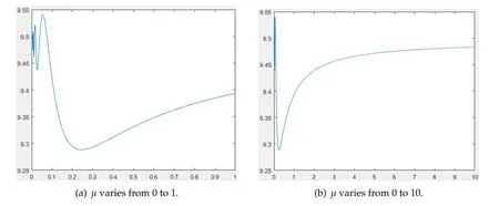
Figure 5
4 Discussions
In this paper,we investigated a diffusive predator-prey model in spatially inhomogeneous environments subject to zero Neumann boundary conditions.In contrast to spatially homogeneous environments,the local dynamics of the model in spatially inhomogeneous environments is more complicated.It turns out that for some ranges of the death rate of the predator,the semi-trivial steady state of this model in spatially heterogeneous environments can change its stability at least once as the dispersal rates of the predator and prey vary,whereas in spatially homogeneous environments,the stability of the semi-trivial steady state of this model is irrelevant to the dispersal rates of the predator and prey.These results have significant implication in ecology.A change in dispersal rates of the predator and prey can alter the influences and consequences of interactions of different organisms.
For a more generalized predator-prey model in spatially heterogeneous environments:
wherer(x)is the intrinsic growth rate of the prey and depends upon the spatial variablex.It is of importance to inquire the stability of the semi-trivial steady state (u*,0) of(4.1) as it determines whether the predator can successfully invade when rare,whereu*=u*(x,μ)is the unique positive solution of
The stability of(u*,0)has been examined in[14,Theorem 1.1]withr(x)=c1K(x)and in Theorem 1.1 withr(x)=c2for some constantsc1,c2>0,respectively.However,due to the limitations of current mathematical methods,it is difficult to acquire the stability of(u*,0)for the general model(4.1).One of the key ingredients is that the structure of
is unclear.
The limiting behaviors ofF(μ) asμtends to zero and infinity have been obtained in [3],however,the diagram ofF(μ) is still vague.To further understand the structure ofF(μ),we shall adopt numerical simulation to predict howF(μ) changes asμvaries from small to large.In the following figures,the vertical coordinate denotesF(μ)and the horizontal coordinate representsμ.Since the graphic ofF(μ) enormously depends onrandK,we consider the following three cases:
(i)ris a function ofK,i.e.,r(x)=h(K(x)) for some functionh,andh/Kis strictly decreasing inK.
In this case,we chooseK(x)=x+9 andr(x)=forx∈Ω=(0,1).By some simple computations,we derive
From Fig.5(a)and(b),we see that there exist several maximum and minimum ofF(μ).Moreover,the diagram ofF(μ)oscillates wildly around 9.5 nearμ=0.In comparison with the casesr(x)=c1K(x)andr(x)=c2forc1,c2>0,the shape ofF(μ)is more complicated.
(ii)ris a function ofK,i.e.,r(x)=h(K(x)) for some functionh,andh/Kis strictly increasing inK.In Fig.6,we selectK(x)=x+9 andr(x)=(x+9)(x+10)forx∈Ω=(0,1).It is easy to show
Fig.6 (a) and (b) can be used to characterize the change rule ofF(μ) asμvaries from smaller and bigger scale,respectively.
(iii)ris a function ofK,i.e.,r(x)=h(K(x)) for some functionh,buth/Kis nonmonotone with respect toK.In this case,it turns out that the image ofF(μ) is more complicated.In Fig.7,we chooseK(x)=x+9 andr(x)=(x+9)forx∈Ω=(0,1).Some calculations yield
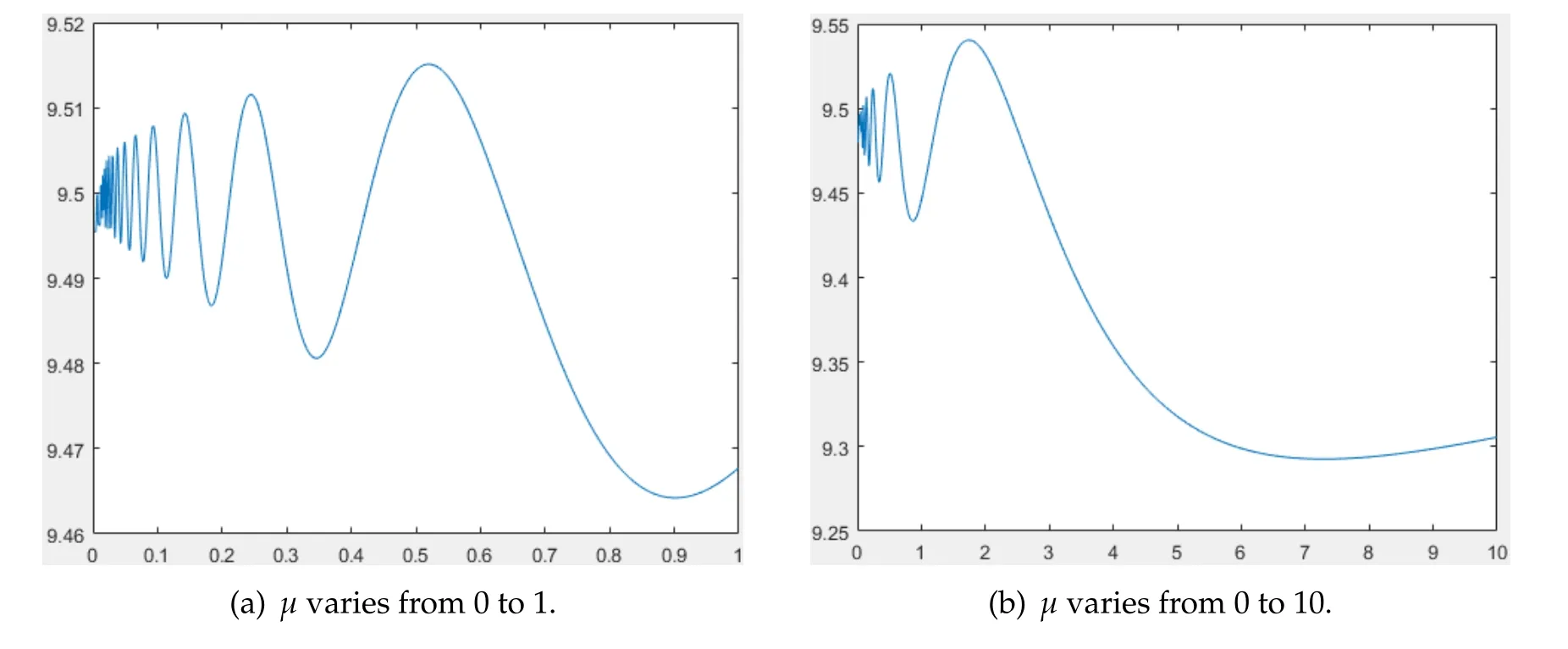
Figure 6

Figure 7
In Fig.8,we selectK(x)=x+9 andr(x)=(x+9){sin[2π(x+9)]+1}forx∈Ω=(0,1).In addition,For this case,the quantitative relation between limiting values ofF(μ)asμtend to zero and infinity is uncertain.Furthermore,there are multiply maximum and minimum ofF(μ)forμ∈[0,∞].To more precisely investigate how(u*,0)of(4.1)changes its stability asμandνvary,the death ratedof the predator should be classified into several cases according to the maximum and minimum ofF(μ).
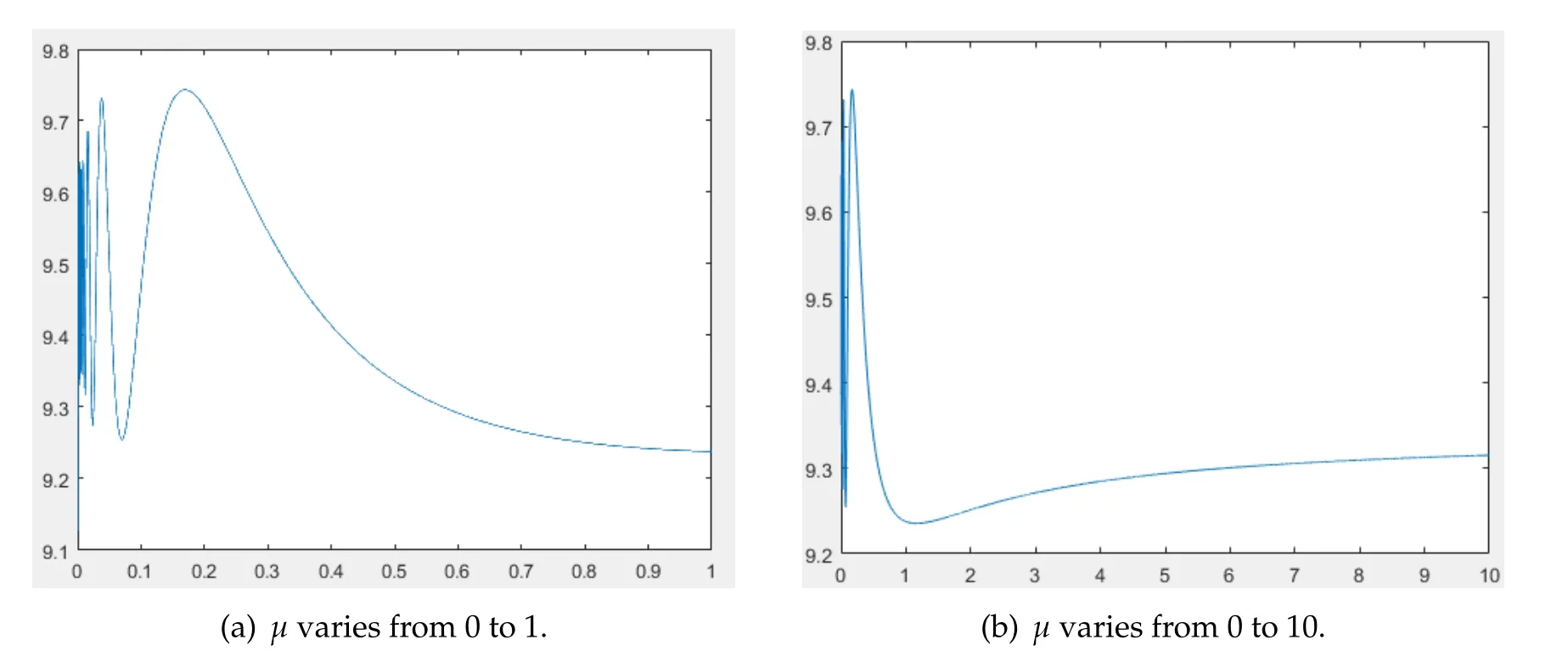
Figure 8
We applied numerical simulation to predict the shape ofF(μ),which is closely related to the stability of (u*,0).Hence,appropriate assumptions onr(x) andK(x) should be explored.On the other hand,other topics concerning such as existence and multiplicity of positive steady states of(4.1)will be considered in the future.
Acknowledgement
This work was supported by the National Science Foundation of China(No.11801436).
 Journal of Partial Differential Equations2023年4期
- Journal of Partial Differential Equations的其它文章
- Modified Differential Transform Method for Solving Black-Scholes Pricing Model of European Option Valuation Paying Continuous Dividends