Mapping Seismic Hazard for Canadian Sites Using Spatially Smoothed Seismicity Model

Chao Feng · Han-Ping Hong

Abstract The estimated seismic hazard based on the delineated seismic source model is used as the basis to assign the seismic design loads in Canadian structural design codes.An alternative for the estimation is based on a spatially smoothed source model.However, a quantif ication of dif ferences in the Canadian seismic hazard maps (CanSHMs) obtained based on the delineated seismic source model and spatially smoothed model is unavailable.The quantif ication is valuable to identify epistemic uncertainty in the estimated seismic hazard and the degree of uncertainty in the CanSHMs.In the present study, we developed seismic source models using spatial smoothing and historical earthquake catalogue.We quantif ied the dif ferences in the estimated Canadian seismic hazard by considering the delineated source model and spatially smoothed source models.For the development of the spatially smoothed seismic source models, we considered spatial kernel smoothing techniques with or without adaptive bandwidth.The results indicate that the use of the delineated seismic source model could lead to under or over-estimation of the seismic hazard as compared to those estimated based on spatially smoothed seismic source models.This suggests that an epistemic uncertainty caused by the seismic source models should be considered to map the seismic hazard.

Keywords Adaptive kernel smoothing · Fixed kernel smoothing · Ground motion model · Probabilistic seismic hazard analysis · Seismic hazard map · Uniform hazard spectra

1 Introduction

Probabilistic seismic hazard analysis (PSHA) is usually carried out based on the framework described in Cornell ( 1968)and Esteva ( 1968).The analysis requires consideration of the seismic source model, magnitude-recurrence relation,and attenuation relation (that is, the ground motion prediction equation or ground motion model).The framework can be illustrated in a logic tree if combinations of the source zone, magnitude-recurrence relation, and ground motion model are considered, where the estimation of the seismic hazard is performed by folding the tree by applying the total probability theory (McGuire 2004).This can be carried out by using the numerical integration technique (McGuire 2004) or simulation technique (Musson 2000; Hong et al.2006).The seismic hazard assessment results are important for seismic structural reliability analysis and the selection of optimal seismic design (Rosenblueth 1976; Goda and Hong 2006; Hong and Hong 2007).

Many advances have been reported on the assignment of the source model, modeling and characterizing magnitude-recurrence relations, and the development of ground motion models.The advances include a better understanding of the earthquake occurrence mechanism, the ground motion characteristics, and the statistical techniques used to develop the source model, the frequency distribution of the magnitude and the occurrence rate, and the ground motion models (Gerstenberger et al.2020).The history of the application of the PSHA framework to estimate Canadian seismic hazard maps (CanSHMs), which were implemented in Canadian structural design codes, was presented in Adams ( 2019) (see also Hong et al.2006).According to Adams ( 2019), Natural Resources Canada (NRCan) (and its predecessors) has been responsible for six generations of seismic hazard maps for Canada since 1953.The mapped Canadian seismic hazard formed the basis for the seismic design provisions recommended in the National Building Code of Canada (NBCC).These studies pointed out that the last three generations of CanSHMs are developed based on a source model that consists of a set of delineated source zones.The source model def ined by a set of source zones(Kolaj et al.2019; Kolaj et al.2020) was used to develop the 6th generation of CanSHM.

The boundary of each source zone could be determined using existing geological or geophysical knowledge.Each source zone is assumed to have similar seismicity characteristics.However, def ining the boundary may introduce uncertainty and could potentially involve a circular argument (Hong et al.2006).The use of spatially smoothed seismic source models (that is, seismic source model obtained based on the historical earthquake catalogue and spatial smoothing techniques) was considered by several researchers (Kagan and Jackson 1994; Frankel 1995; Woo 1996;Stock and Smith 2002; Hong et al.2006; Xu and Gao 2012;Feng and Hong 2021).The smoothed seismic source model is obtained by spatially smoothing the historical earthquake occurrence using a kernel function with a f ixed or adaptive bandwidth.The smoothing of the spatial occurrence could be carried out by neglecting or considering the earthquake magnitude dependency (Frankel 1995; Woo 1996).

By considering the ground motion models used to develop the 4th generation of CanSHM, Hong et al.( 2006) showed that the degree of smoothing af fects the estimated seismic hazard.The smoothing in their study was carried out using the Voronoi polygon or the spatial kernel smoothing with a constant bandwidth, and the seismic hazard assessment was carried out only for two regions in Canada.Systematic quantif ication of dif ferences in the estimated and mapped seismic hazard at Canadian sites that are obtained based on the delineated seismic source model and spatially smoothed seismic source models, however, is unavailable, although the quantif ication is valuable to identify epistemic uncertainty in the estimated seismic hazard.One may argue that the use of the spatial smoothing approach could not incorporate geological and tectonic features while the use of the delineated source modeling approach is often related to the subjective def inition of the seismic source zones.However, the latter was refuted by arguing that a circular argument exists between the selection of seismicity patterns and the shape of tectonic plates (Hong et al.2006).Therefore, both modeling approaches are valid for seismic hazard modeling and a comparison of the results obtained from these approaches is necessary to quantify their dif ferences.

Note that the ground motion models used for the mapping of the 5th and 6th generations of CanSHMs (denoted as Can-SHM5 and CanSHM6) dif fer.The ground motion models used for CanSHM6 were summarized in Kolaj et al.( 2020).They also indicated that dif ferent software was used for the seismic hazard assessment for CanSHM5 and CanSHM6.

The main objectives of the present study are (1) to map the Canadian seismic hazard by applying the spatially smoothed source models and (2) to quantify the differences between CanSHM6 and that obtained by using the spatially smoothed source models.For consistency, in all cases, the ground motion models used to develop CanSHM6 are adopted in the present study for the seismic hazard assessment.We used two approaches to develop the spatially smoothed source models.The f irst one uses the kernel smoothing technique with a constant bandwidth and the second one uses the adaptive kernel smoothing technique.In both cases, the smoothing was carried out by considering the earthquake magnitude dependency.The considered historical earthquake catalogue, kernel function, and estimation of the bandwidth are described in the following section.This is followed by the description of the estimation and mapping of the seismic hazard and the comparison of the estimated seismic hazard.

2 Application of Spatial Smoothing Techniques to Develop Smoothed Seismic Source Models

In this section, we summarize the historical earthquake catalogue used in the present study.Based on such a catalogue,we develop the spatially smoothed seismic source model by using f ixed as well as adaptive kernel smoothing techniques.Moreover, we compare the magnitude-recurrence relation obtained based on the spatially smoothed source models to that obtained based on the delineated seismic source model that was used for the development of CanSHM6.

2.1 Historical Earthquake Catalogue and Its Completeness Assessment

The historical earthquake catalogue for developing the spatially smoothed source model in the present study is from the 2011 Canadian Composite Seismicity Catalogue (CCSC).1See https:// www.seism otool box.ca/ Docum ents/ ccsc1 1west.txt,https:// www.seism otool box.ca/ Docum ents/ ccsc1 1east.txt.The catalogue consists of the 2011 CCSC West Catalogue and the 2011 CCSC East Catalogue.The 2011 CCSC West Catalogue contains a list of 34,934 historical seismic events that occurred from January 1700 to December 2010, where the epicentral location of each event was within the latitude and longitude of 43.5° N–75° N and 160° W–110° W.The 2011 CCSC East Catalogue contains a list of 11,893 events that occurred from January 1534 to December 2010, where the epicentral location of each event was within the latitude and longitude range of 35° N–80° N and 110° W–45° W.The consideration of this catalogue rather than a more up-to-date catalogue is justif ied since Adams et al.( 2019)indicated that the (delineated) seismic source model used in CanSHM6 remains mostly the same as that used in Can-SHM5, which was developed by considering the seismic events that occurred before 2011 (Halchuk et al.2015), and that the estimated seismic hazard is relatively insensitive to the additional seismic events since the development of the source model used in CanSHM5.In other words, the use of CCSC facilitates the comparison of the assessed seismic hazard obtained by using the delineated seismic source model and the spatially smoothed source model, which are developed based on the same historical seismic catalogue.

For each event, the catalogue provides the occurrence time (year/month/day/hour/minute), epicentral location(latitude and longitude), focal depth (km), magnitudes (for example, body wave magnitudeMb, Nuttli magnitudeMN,local magnitudeML, surface wave magnitudeMS, coda magnitudeMC , duration magnitudeMD , and moment magnitude M), and the original catalogues that reported the event.In the catalogue, M is used as the most preferred magnitude,and the reported Modified Mercalli Intensity (MMI) is adopted to estimate M for early earthquake events due to the unavailability of seismic instruments.M is used for the present study.The historical seismic events that occurred within the spatial coverage, including those that occurred outside of Canada but within about 500 km distance of the Canadian border, are employed to develop the spatially smoothed source model and shown in Fig.1.

A detailed explanation of CCSC was given by Fereidoni et al.( 2012).The number of induced seismic events in this catalogue is small and with a small magnitude.Since according to Halchuk et al.( 2015), the removal of such events is dif ficult if not impossible, no attempt was made to remove such events.A preliminary process for the catalogue is carried out in the present study.The earthquake events for the 2011 CCSC East Catalogue and 2011 CCSC West Catalogue with occurrence time earlier than 1660 and 1860 are removed based on the f irst year of complete coverage for time-magnitude categories (Hong et al.2006).Note that the historical earthquake catalogue is associated with unequal observation periods for different earthquake magnitude intervals.This af fects the evaluation of the magnitude-recurrence relation (Weichert 1980).However, the unequal observation periods are unknown and must be assessed through the completeness analysis (Albarello et al.2001).For the assessment, consider that the catalogue is reported up to the most recent timeT R, and the earliest time when an event with M greater than or equal to a threshold magnitude MTisT MT,S.Let ?Tmax=T R?T MT,Sdenote the maximum observation period for the considered MT.The completeness analysis of the catalogue for events with magnitude greater than Mmin,jsince or after the timeT C,j, forj= 1, …,N C, is to be carried out, whereN Cis the total number of lowest magnitude cases considered for completeness analysis, andT C,j[T R,T MT,S).Given Mmin,j, ΔT C,j=T R?TC,jis divided into 2Nelementary non-overlapping subintervals of equal durationδt= ΔT C,j/(2N), and that a comparison of the earthquake occurrence rates in thei-th and (N+i)-th intervals, denoted asλ iandλ N+i, is carried out.According to Albarello et al.( 2001), the probability of completeness of the catalogue fora given value ofT C,j(that is, within the specif ic time span ΔT C,j),Pj(C|||TC,j) , is given by:′

Fig.1 Spatial distribution of historical earthquake events with M ≥ 3.0, where the red and blue color symbols denote the events reported in the East Catalogue and West Catalogue,respectively

Fig.2 Curves corresponding to p = 0.25, 0.50, and 0.75 for selected events by considering a the CCSC 2011 East Catalogue and b the CCSC 2011 West Catalogue

in whichNj,pis the total number of likely valuestC,j,pto be considered.tC,j,pis considered as the point estimate ofT C,j.The inter-quantile range, |tC,j,0.25?tC,j,0.75| , is used as a measure of the uncertainty inT C,j.It is further assumed thatTC,j>TC,kfor M min,j< M min,k.For the numerical analysis to be carried out,Nis set equal to 120,?is taken equal to 1.5,the values ofpequal to 0.25, 0.5, and 0.75 are considered(Feng et al.2020), and M ranging from 3 to 7.25 and 3 to 8.0 is considered for completeness analysis of 2011 CCSC East Catalogue and 2011 CCSC West Catalogue, respectively.Based on these considerations, the obtainedtC,j,pfor the employed historical seismic events for the CCSC East Catalogue and the CCSC West Catalogue are shown in Fig.2 a and b.

Many source zones are included in the source model for developing CanSHM6 (Kolaj et al.2019).In each source zone, the earthquake is assigned to one of the f ive earthquake types: (1) stable crustal earthquake, (2) active shallow crustal earthquake, (3) subduction inslab earthquake with focal depth greater than 30 km (which is referred to as subduction inslab30), (4) subduction inslab earthquake with a focal depth greater than about 55 km (which is referred to as Subduction Inslab55), and (5) subduction interface earthquake; these earthquake types will be simply referred to as type 1 to 5, respectively.By considering these, each of the historical seismic events in the catalogues is assigned an earthquake type according to its geographical location (that is, latitude, longitude, and focal depth) and magnitude.The value ofT C,j,tC,j,p, for an earthquake event with an assigned earthquake type of a magnitude greater than Mmin,jis shown in Fig.2.

Since no interface earthquake could be identif ied from the historical catalogue based on the adopted criteria for the geographical location and magnitude, the spatial smoothing is carried out only based on the remaining four types of earthquakes.Note that the use ofp= 0.5 was by Albarello et al.( 2001).By adopting such a value, the earthquake events identif ied based on the completeness analysis (that is, earthquakes within the completed catalogue) are shown in Fig.3.A comparison of the results shown in Figs.1 and 3 indicates that the number of seismic events shown in Fig.3 is much less than that shown in Fig.1 and that the seismic activity varies geographically.The earthquakes within the completed catalogue forp= 0.5 is used in this study for developing the spatially smoothed source models.

2.2 Spatially Smoothed Seismic Source Models

In the present study, both the f ixed kernel smoothing technique and adaptive kernel smoothing technique are considered to develop the spatially smoothed seismicity.The area within Canada is covered by a grid system with 0.5° × 0.5°(latitude × longitude) cells.For the f ixed kernel smoothing technique, the smoothing procedure given by Woo ( 1996)is followed.Woo ( 1996) used the following kernel functionK(＆#x1d40c;i,j,x?xi,j) (Vere-Jones 1992):

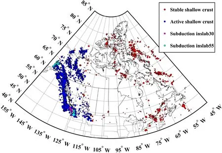
Fig.3 Historical seismic events that are identif ied based on the earthquakes within the completed catalogue for p = 0.5

wherea1,ianda2,iare the model parameters.These model parameters are estimated based on regression analysis by using one of the following three options and the earthquakes within the completed catalogue with M ≥ 3.0, which are grouped in bins according to the value of earthquake magnitude where the bin width equal to 0.25 is used in all cases.Option 1 follows the procedures suggested by Molina et al.( 2001), where the earthquake events are grouped according to the number of bins of earthquake magnitude, and the pair of samples for each bin is formed by using the magnitude at the center of the bin and the shortest spatial distance between any pair of events within the bin.The samples are presented in Fig.4 and are used for regression analysis based on Eq.5.The f itted curve is also shown in Fig.4.Rather than carrying out regression analysis based on Option 1, in Option 2, the regression is carried out by using the average of the shortest distance from a given event to any other events within the bin (Zuccolo et al.2013).The samples as well as the f itted curve based on this option are also shown in Fig.4.In Option 3, as suggested by Goda et al.( 2013), the magnitude of each seismic event within a bin and its shortest distance to any event within the bin is used as a paired sample.The collection of the samples, as well as the f itted curve based on the parametric model shown in Eq.5 for the considered seismic events within the completed catalogue, are shown in Fig.4.In general, the f itted curves based on Option 3 are between the curves determined based on Options 1 and 2.Therefore, the f itted model based on Option 3 is considered in the following for the numerical analysis.

Before carrying out the spatial smoothing for the development of the seismic source models, we plot the historical seismic events within the completed catalogue with the magnitude M greater than Mmin= 4.8 as shown in Fig.5.This Mmin= 4.8 is the same as that adopted for the development of CanSHM6 (Kolaj et al.2020).Based on the adopted kernel function shown in Eq.4 and the bandwidth shown in Eq.5, the smoothed magnitude-recurrence relation based on the f ixed kernel smoothing technique for thek-th cell with magnitude greater than M by considering thei-th earthquake type, denoted asλ F,i,k( M) per year and per km 2 , is evaluated according to:

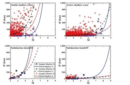
Fig.4 Samples and f itted curves are def ined by Eq.4 by considering three dif ferent options

Fig.5 Historical earthquake events within the completed catalogue with M ≥ 4.8

Fig.6 The plotted values are the rates per cell (0.5° × 0.5°) rather than per unit area: a λ F,K ( M min ) and b λ A,k ( M min ) based on M min = 4.8.The squares shown in the plots indicate the location of the identif ied sites to be considered

whereI(＆#x1d40c;i,j≥＆#x1d40c;) is an index function that equals 1 for Mi,j≥ M and zero otherwise,E jdenotes the earthquake type for thej-th event, which can be 1, 2, 3, or 4,IE(Ej=i) is an index function that equals 1 forEj=iand zero otherwise,N Tis the total number of earthquakes in the completed catalogue considered,xkis the center of thek-th cell, and ΔtC,j,0.5=TR?tC,j,0.5.The sum ofλ F,i,k( Mmin) fori= 1 to 4, denoted asλ F,k( Mmin), represents the occurrence rate by considering all four earthquake types.

The adaptive kernel smoothing technique is also considered.For the adaptive kernel smoothing technique, the local bandwidth for thek-th cell with a magnitude greater than M is:

wheren c,iis the total number of the cells that cover the area within Canada fori-th earthquake type andγis a model parameter that is taken as equal to 0.5 (Silverman 1986).By using the estimatedci,k(＆#x1d40c;) , the magnitude-recurrence relation for thei-th earthquake type and thek-th cell,λ A,i,k( M),is given:that occurred in eastern Canada, and a smoother seismicity is observed for western Canada.Bothλ F,k( Mmin) andλ A,k( Mmin) follow the spatial distribution of the historical earthquake events, andλ F,k( Mmin) for cells in the Cascadia subduction area is greater thanλ A,k( Mmin).The parameters used for spatial smoothing are given in Table 1.These parameters were determined based on the procedure given by Goda et al.( 2013).In the same table, we also included the estimated total occurrence rate by considering each earthquake type for M ≥ 4.8.The obtained rate based on the f ixed kernel smoothing,＆#x1d706;TF,k(4.8) , is the same as that obtained by using the adaptive kernel smoothing,＆#x1d706;TA,k(4.8).

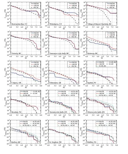
To appreciate the magnitude-recurrence relation, we plot the estimatedλ F,k( M) andλ A,k( M) in Fig.7 for 15 selected representative sites that are identif ied in Fig.6(squares).The results presented in Fig.7 indicate that the trend observed fromλ F,k( M) agrees well with that fromλ A,k( M).Overall,λ A,k( M) for the considered sites is greater thanλ F,k( M).For four sites, Vancouver, Kelowna,Whitehorse, and Destruction Bay, there are appreciable

The sum ofλ A,i,k( Mmin) fori= 1 to 4, denoted asλ A,k( Mmin), represents the occurrence rate by considering all four earthquake types that are obtained based on the adaptive kernel smoothing.Based on the above, the calculatedλ F,k( Mmin) andλ A,k( Mmin) are shown in Fig.6 a and b,respectively (log represents the logarithm with base 10).Figure 6 shows thatλ A,k( Mmin) is more concentrated thanλ F,k( Mmin) for regions with concentrated historical eventsdif ferences betweenλ F,k( M) andλ A,k( M).A further inspection of the results indicates that such a discrepancy is due to the use of a narrower bandwidth in the adaptive kernel smoothing as compared to that in the f ixed kernel smoothing.

Table 1 Bandwidth parameters used for smoothing and total occurrence rate by considering each earthquake type

Fig.7 Estimated λ F, k ( M) and λ A, k ( M) per 0.5° × 0.5° cell based on M min = 4.8 for 15 representative sites.The square, cross, and triangle are used in the plots to indicate M obs for earthquake types 1, 2, and 4.FKSM and AKSM denote f ixed kernel smoothing technique and adaptive kernel smoothing technique, respectively

The maximum magnitude, denoted as Mobs, in the estimatedλ F,k( M) andλ A,k( M), as shown in Fig.7 for each site,is directly controlled by the observed maximum magnitude for the earthquakes in the completed earthquake catalogue.They are equal to 7.40, 8.45, 6.10, and 7.00, for the earthquake type 1 to 4 (that is, eastern stable crustal earthquake,western active shallow crustal earthquake, subduction inslab earthquake with focal depth greater than 30 km, and subduction inslab earthquake with focal depth greater than about 55 km), respectively.These values can be smaller than the central values of the maximum magnitude adopted in developing CanSHM6, which are 7.8, 8.27, 7.00, and 7.60, for the earthquake type 1 to 4, respectively.Therefore, as a conservative measure, we consider that the maximum magnitude,M max , values for the four types of earthquakes are equal to the maximum of the mentioned two sets of values.In addition, if the maximum comes from Mobs, an additional 0.1 is included as a conservative measure.That is, Mmaxequal to 7.80, 8.55, 7.00, and 7.60 for the four types of earthquakes are employed in the PSHA carried out in the following.

For cases where Mobsis less than Mmaxfor thei-th earthquake type, the magnitude-recurrence relation for M greater than Mobsis modeled using:

in which the regression analysis is employed to estimateβ kusing the magnitude-recurrence relation for M up to Mobsthat is determined for thek-th cell based on the f ixed kernel smoothing technique.Similarly,λ A,i,k( M) for M ≥ Mobs,is def ined by using Eq.9, except that the subscriptFis replaced byAandβ kis determined based on the magnituderecurrence relation determined for thek-th cell based on the adaptive kernel smoothing technique.

Since the assessed seismic hazard for a site of interestxis mainly dominated by the earthquakes that occurred at a distance to this site smaller than 250 km (Goda and Hong 2009), it is instructive to estimate and compare the seismic occurrence rate in a circle centered at the site of interest with a radius equal to 250 km by considering dif ferent seismic source models.We evaluate such a rate, denoted asλ250km( M), by integrating the magnitude-recurrence rate within the circle for the site of interest by considering the source model adopted in developing CanSHM6 (which is referred to as CanSSM6), the source model developed by the f ixed kernel smoothing technique (FKSM), and the source model developed by the adaptive kernel smoothing technique (AKSM).The obtained values ofλ250km( M)for a few selected sites are shown in Fig.8.In general,the rate shown in Fig.8 obtained by considering FKSM is similar to that obtained by considering AKSM.However,a relatively large discrepancy is observed for Whitehorse,Kelowna, Calgary, and Edmonton.This is attributed again to the bandwidth used in these two smoothing techniques.

Note that CanSSM6 consists of three regional seismic source models that cover the regions in Canada (Kolaj et al.2020).These three regional models are the Western Canada model, the Eastern Arctic model with two submodels (H2 and R2 with weights equal to 0.6 and 0.4,respectively), and the Southeastern Canada model with three sub-models (H2, HY, and R2 with weights equal to 0.4, 0.4, and 0.2, respectively).For each sub-model, the nine magnitude-recurrence relations (with three sets of magnitude-occurrence rate models in combination with three values of Mmax), each with its associated probability,are considered.By folding the logical tree representing the source models, the overall magnitude-recurrence relation was developed and used as the input to develop Can-SHM6 by using OpenQuake (Pagani et al.2014).We use such an overall magnitude-recurrence relation to evaluateλ250km( M) for the considered sites of interest as shown in Fig.8.The comparison shown in Fig.8 indicates that the estimatedλ250km( M) for sites located in western Canada by using FKSM and AKSM is relatively greater than that obtained based on the seismic source model adopted for the development of CanSHM6.This is especially the case for M greater than about 6.5.For sites located in eastern Canada, the estimatedλ250km( M) by dif ferent methods are more comparable.Therefore, it is expected that the estimated hazard by using dif ferent seismic source models is likely to result in dif ferent seismic hazard estimates.The quantif ication of the dif ferences in the estimated seismic hazard is presented in the following sections.

3 Seismic Hazard Assessment

First, we describe the ground motion models (GMMs) that were used for CanSHM6 and adopted in the present study.We then present the adopted simulation procedure used for seismic hazard assessment based on the delineated or spatially smoothed seismic source models.We estimate the seismic hazard as well as the uniform hazard spectrum for a few selected sites by using dif ferent seismic source models.

3.1 Ground Motion Models Used for the Development of CanSHM6

Before carrying out PSHA by using the developed FKSM and AKSM, we brief ly summarize the GMMs adopted for developing CanSHM6 (Kolaj et al.2019).For eastern stable shallow crustal earthquakes, two sets of GMMs are adopted,each with a probability of 0.5.The f irst set of GMMs was given by Atkinson and Adams ( 2013), hereafter AA13.This set was developed for eastern stable crustal earthquakes; it included three GMMs (or three GMM curves) to account for the epistemic uncertainty.These three were termed “upper,”“central,” and “lower” GMMs with associated weights equal to 0.25, 0.50, and 0.25, respectively.The central GMM in AA13 is constructed by taking the arithmetic average of the f ive candidate GMMs: one from Pezeshk et al.( 2011), one from Atkinson and Boore ( 2011), one from Atkinson ( 2008)and Atkinson and Boore ( 2011), and two from Silva et al.( 2002) for eastern North America.The upper and lower GMM curves are obtained by ± the standard deviation (in the logarithmic scale), each with a weight of 0.25, and the central GMM represents the median curve with a weight of 0.50.The second set, which is based on the Central and Eastern North America project, was given by Goulet et al.( 2017), hereafter Gea17.The Gea17 is obtained by weighing a set of 13 candidate GMMs by using weights that depend on the natural vibration periodT n; the standard deviation for Gea17 is the same as that for AA13.Note that Kolaj et al.( 2020) considered that the standard deviation for Gea17 is the same as that for AA13.Although it would be interesting to investigate the impact of the assumed standard deviation on the estimated seismic hazard, this is beyond the scope of the present study.

The four sets of GMMs given by the NGA-West2 project (Abrahamson et al.2014; Boore et al.2014; Campbell and Bozorgina 2014; Chiou and Youngs 2014), hereafter ASK14, BSSA14, CB14, and CY14, each with a weight of 0.25, are employed for western active shallow crustal earthquakes.

?

The GMMs given by Atkinson and Boore ( 2003),Abrahamson et al.( 2016), García et al.( 2005), and Zhao et al.( 2006), hereafter AB03, Aea16, Gea05, and Zea06,are adopted for subduction inslab earthquakes; and the GMMs given by Abrahamson et al.( 2016), Atkinson and Macias ( 2009), Ghofrani and Atkinson ( 2014), and Zhao et al.( 2006), hereafter Aea15, AM09, GA14, and Zea06,are considered for subduction interface earthquakes.The weights assigned for each of the four GMMs for subduction inslab are 0.25.The same is done for the GMMs for subduction interface earthquakes.

The predicted median of the peak ground acceleration(PGA), spectral acceleration (SA) at the natural vibration period,T n= 0.2, 0.5, and 2 s forVS30= 450 m/s based on the adopted GMMs for CanSHM6 (Kolaj et al.2020) is illustrated in Fig.9.In the f igure,δis the fault dip,?is the strike angle,λis the rake angle,L Ris the rupture length,W Ris the rupture width,R a=L R/W R,H SUis the upper seismogenic depth,H SLis the lower seismogenic depth,andF his the focal depth.The geometric representation of these parameters is depicted in Fig.10.

For the predicted PGA and SA values presented in the f igure for a given scenario event def ined byM,δ,?,λ,R a,H SU, andH SL, the rupture area,Arup, is calculated using the following rupture scaling relationship:

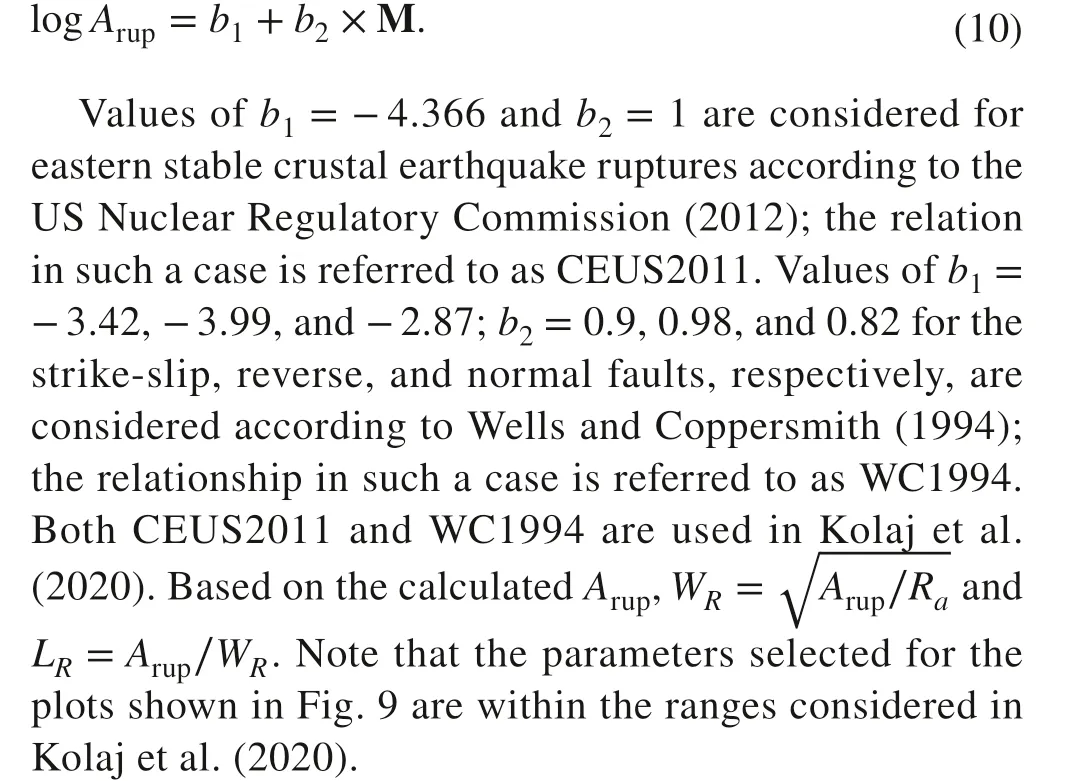
Figure 9 shows that the relative variability for the predicted median ground motion is increased with the increasedT n.Also, an increased variability for the predicted PGA and SA by using different GMMs for a scenario event is observed as the distance to the rupture surface decreases and the magnitude increases.

3.2 Procedure Used for Probabilistic Seismic Hazard Analysis (PSHA)

The GMMs, which were described in the previous section and adopted for developing CanSHM6, are used in the following for the PSHA by considering FKSM and AKSM.The procedure for carrying out PSHA is based on the simulation steps given by Hong et al.( 2006).For comparison purposes,we also considered CanSSM6.In this case, rather than using OpenQuake, we also use the same simulation procedure for consistency.The major steps for the simulation procedure include: (1) sample earthquake occurrence according to the adopted stochastic model for each earthquake type (for example, Poisson process); (2) generate the magnitude based on the considered earthquake type and magnitude-recurrence relation for each sampled seismic event; (3) sample rupture geometry parameters for each seismic event based on the corresponding probability distribution models as describe in CanSHM6 (see Tables 2 and 3); (4) evaluate the ground motion measures (that is, PGA and SA) at a site of interest by using the adopted GMMs; and (5) extract the annual maximum of PGA or SA to form their empirical probability distributions that can be used to estimate theT-year return period value of PGA,A T, and of SA,S T(T n).In all cases, the analysis is carried out using the adopted GMMs forVS30=450 m/s, which was considered for CanSHM6.

3.3 Comparison of the Estimated Site-Specif ic Seismic Hazard

Seismic hazard assessment is carried out by using the procedure, the source models (CanSSM6, FKSM, and AKSM), and the GMMs described and summarized in the previous sections.The consideration of CanSSM6 is for comparison purposes.For the analysis, one million years of seismic activities are simulated.Based on the analysis results, the empirical probability distribution of the annual maximum PGA in the upper tail region is shown in Fig.11.The figure shows that the probability distribution of the annual maximum PGA in the upper tail region can be adequately modeled as a lognormally distributed random variable.The fact that the distributions in each plot do not have the same slope indicates that the magnitude of the uncertainty of the annual maximum PGA in the upper tail depends on the considered seismic source model.In several cases, the distributions are separate, suggesting that the estimated return period value of the annual maximum PGA for a site differs by considering different source models.Depending on the considered site, the large difference in the distribution could be between those obtained by using CanSSM6 and FKSM, by using CanSSM6 and AKSM, or by using FKSM and AKSM.In addition, a simple analysis indicates that the value of the coefficient of variation based on the fitted distribution to the upper tail region varies spatially.For example, it is about 2 for Vancouver and Victoria; ranges from about 5 to 9 for Ottawa, Montreal,and Quebec, and is greater than about 10 for Edmonton,Winnipeg, Toronto, Halifax, and St.John’s.The observed large spatial variation is consistent with that indicated in Hong et al.( 2006).Although the spatially varying coefficient of variation could have a significant impact on the development of reliability-consistent or risk-target seismic design maps for Canadian sites (Hong and Hong 2006), the investigation of this topic is beyond the scope of the present study.

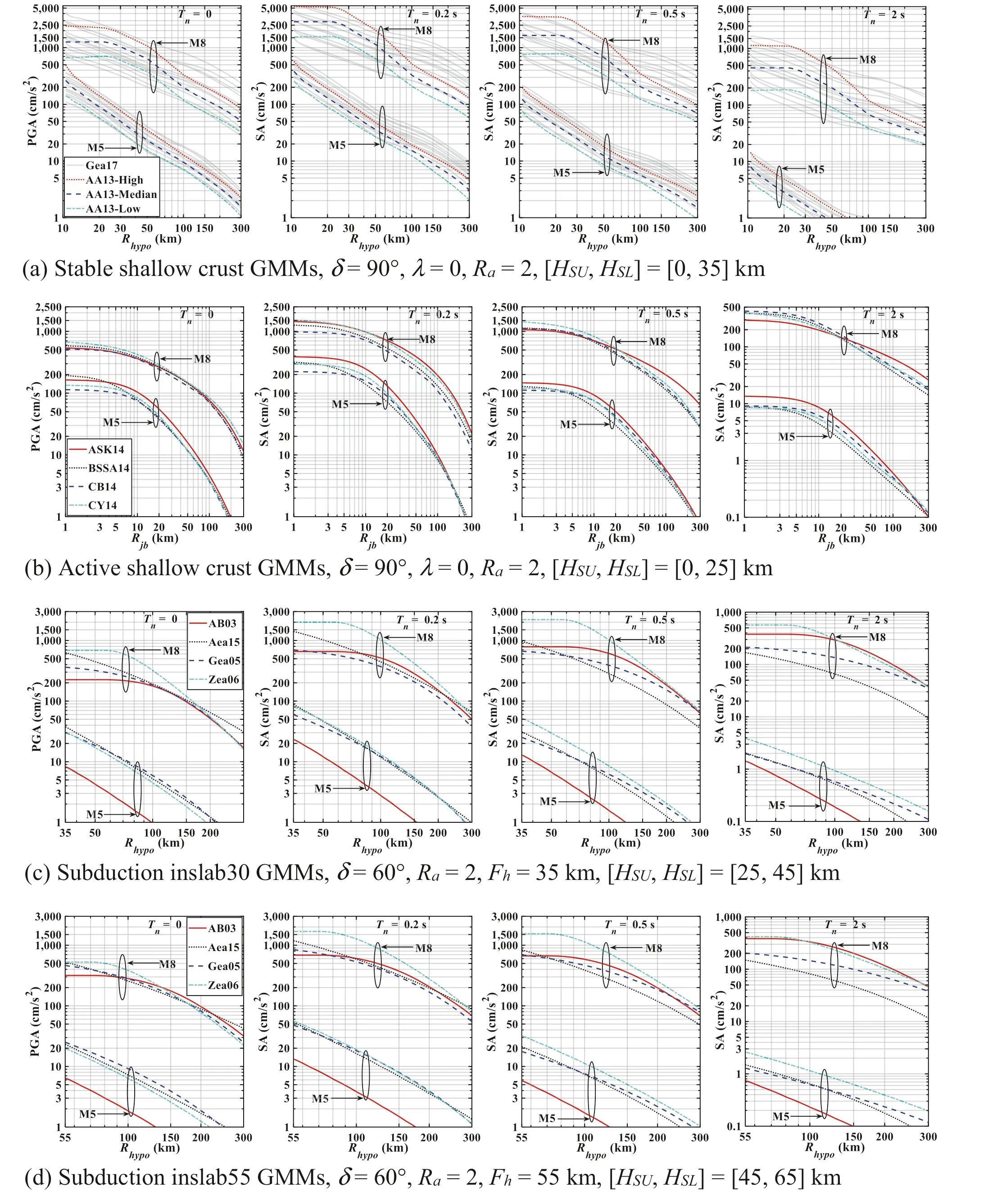
Fig.9 Ground motion models (GMMs) used to estimate the seismic hazard by considering peak ground acceleration (PGA), and spectral acceleration (SA) at T n = 0.2, 0.5, and 2 s for the four considered earthquake types

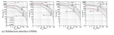
Fig.9 (continued)

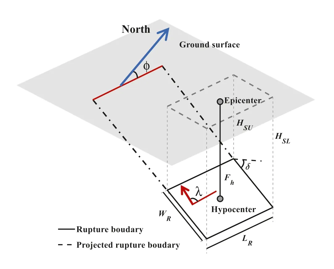
Fig.10 Representation of the earthquake rupture plane

To better appreciate the dif ference in theT-year return period of the annual maximum PGA,A T, we estimateA2475(that is, quantile with an exceedance probability of 2% in 50 years) from the empirical distributions shown in Fig.11.We show the estimatedA2475in Table 4.We include the values reported by Kolaj et al.( 2020) (that is, from CanSHM6) in the table as well for comparison purposes.In addition, we also plot the empirical distribution for annual maximum SA at the vibration periodT n,denoted asS(T n), forT n= 0.2 and 2.0 s.Since the observed trends are similar to those shown in Fig.11, they are not included (to save space).However, the estimatedT-year return period values ofS(T n),S T(T n), from the empirical distribution are shown in Table 4 forT= 2475 years, andT n= 0.2 and 2.0 s.Similarly, for comparison purposes,

Table 2 Distribution models for ?, δ, and λ (in degrees) for seismic events with dif ferent tectonic settings for spatially smoothed seismicity model[values used for CanSHM6 are from Kolaj et al.( 2020)]

Table 3 Distribution of H hypo , [H SU , H SL ] (value unit: km), and rupture scaling relationship adopted for the considered tectonic regions[values used for CanSHM6 are from Kolaj et al.( 2020)]

Rather than showing the estimatedA TorS T(T n), we plot the estimated uniform hazard spectra (UHS) in Fig.12 for the 23 selected sites by consideringT= 2475 years.In all cases, the trends of the UHS are consistent for considered source models and CanSHM6.Since the logarithmic scale is used for the vertical axis of the plot, the dif ferences in the estimated UHS by using dif ferent source models appear to be relatively small.The UHS from CanSHM6 and the estimated UHS by considering CanSSM6 in the present study agree very well.Also, the estimated UHS by considering FKSM and AKSM are consistent.

4 Seismic Hazard Maps Obtained by Considering Dif efrent Seismic Source Models

we include the reported values ofS2475(T n) by Kolaj et al.( 2020) in Table 4.

To quantify the differences in the predictedA TandS T(T n) shown in Table 4, we def ine the relative dif ferencerA∕B=(yA?yB)∕yB, whereAandBrepresent CanSSM6,FKSM, AKSM, or CanSHM6, respectively, andy ArepresentsA TorS T(T n) by using the source model A, andy Bis def ined similarly.By considering the PGA,rCanSHM6/CanSSM6for the sites withA Tgreater than 0.1granges from ? 7.9 to 7.8% with a mean of practically zero.These values become? 4.6%, 7.6%, and 1.8% by consideringS T(0.2), and ? 1.4%,10.7%, and 2.7% by consideringS T(2.0) ifS T(T n) greater than 0.1gis considered.This comparison indicates that the results obtained by our approach and OpenQuake agree well.

By considering againA TorS T(T n) (for FKSM) greater than 0.1g, the obtained minimum, maximum and mean ofrCanSHM6∕FKSMequal ? 114.3%, 80.4%, and 22.6% for PGA,? 100.1%, 79.7%, and 19.6% forS T(0.2), and ? 90.3%,80.4%, and ? 4.5% forS T(2.0).Similarly, the obtained minimum, maximum, and mean ofrCanSHM6/AKSMequal ? 56.0%,78.4%, and 18.5% for PGA, ? 222.5%, 71.9%, and 7.0% forS T(0.2), and ? 34.7%, 65.9%, and ? 0.2% forS T(2.0) ifA TorS T(T n) (for AKSM) greater than 0.1gis considered.These calculated relative dif ferences ref lect the observed dif ference in the source models.

By considering againA TorS T(T n) (for AKSM) greater than 0.1g, the calculatedrFKSM/AKSMequal ? 107.4%, 30.4%,and ? 8.8% for PGA, ? 280.6%, 27.9%, and ? 20.8% forS T(0.2), and ? 8.1%, 29.2%, and 3.2% forS T(2.0).These results indicate that the obtained seismic hazard by using FKSM and AKSM, on average, are consistent although in some cases there are signif icant dif ferences.Again, these observed dif ferences ref lect the dif ference in the obtained spatially smoothed source models.To map the seismic hazard, we estimateA TorS T(T n) by following the procedure used in the previous section but for each cell of 0.5° × 0.5° in a grid system covering the regions in Canada.In all cases, we considerVS30= 450 m/s,T n=0.2, 0.5, 1, 2, 5, and 10 s, and each of the three source models (CanSSM6, FKSM, AKSM).The obtainedA2475 (that is,S2475(0)) andS2475(0.2) are shown in Fig.13.Note that although we have plotted and inspected the maps for otherT nvalues, they are not included here (to save space).

An inspection of the results shown in Fig.13 indicates that, in general, the spatial trends of the seismic hazard maps obtained by considering dif ferent source models are similar.This is expected as the comparison shown in the previous sections indicates that, on average, the estimatedA TorS T(T n)by considering dif ferent source models are in good agreement.To quantify the dif ferences between dif ferent maps, we calculate the average of the ratio ofS T(T n) obtained by considering FKSM to that obtained by considering CanSSM6.The obtained values forT n= 0, 0.2, 0.5, 1, 2, 5, and 10 s are 0.98, 0.95, 0.97, 0.98, 1.03, 1.15, and 1.21, respectively.This indicates that, on average, the use of CanSSM6 could overestimate or underestimate the seismic hazard as compared to that obtained by using FKSM.We also calculate the average of the ratio ofS T(T n) obtained by considering AKSM to that obtained by considering CanSSM6.The obtained values forT n= 0, 0.2, 0.5, 1, 2, 5, and 10 s are 0.95, 0.95, 0.93, 0.93, 0.95, 1.02, and 1.08, respectively.In this case, the use of CanSSM6 could overestimate the seismic hazard as compared to that obtained by using AKSM,depending on the considered vibration period.Given the absence of compelling justif ications to dismiss the spatially smoothed source models, one may consider multiple seismic source models as part of the logic tree for the seismic hazard assessment.In such a case, one may assign a weight of 0.5 for CanSSM6, 0.25 for FKSM, and 0.25 for AKSM to develop the combined source model.By adopting such a combined source model and repeating the seismic hazard mapping analysis, the obtained maps in terms ofA2475andS2475(0.2) are also shown in Fig.14.The calculated average of the ratio ofS T(T n) obtained by considering the combined source model to that obtained by considering CanSSM6 is 0.98, 0.97, 0.97, 0.98, 0.99, 1.04, and 1.07, forT n= 0, 0.2,0.5, 1, 2, 5, and 10 s, respectively.The average of the ratio indicates that the estimated seismic hazard by considering the combined source model becomes relatively consistent.But this consistency, which is based on average behavior,should not be extended to an individual site.

Fig.11 Empirical probability distributions of annual maximum peak ground acceleration (PGA) for the upper tail region for 23 locations

It must be emphasized that in recent years, the assessment of the seismic hazard due to the induced seismic events caused by hydraulic fracturing was also carried out (Atkinson et al.2015; Atkinson et al.2016).The results indicate that the magnitude-recurrence relation for the induced seismicity and their ground motion attenuation characteristics are dif ferent from the natural seismic events.The studies further showed that the seismic hazard due to the induced seismic events in Alberta, Canada, could be greater than that due to natural hazards.This can be explained by noting that the seismic hazard due to natural seismic events in Alberta is very small.Such seismic hazard is not included in Figs.11,12, 13, and 14.

5 Conclusion

The current Canadian seismic hazard maps are developed by considering a delineated source model (that is, CanSSM6).These maps provide information about theT-year return period values of annual maximum spectral acceleration(SA) at the natural vibration periodT n, referred to as ST(T n),as well as the annual maximum peak ground acceleration(PGA), denoted asA T, represented as ST(T n).

In the present study, we developed two new source models, namely FKSM and AKSM, using the historical earthquake catalogue and employing the f ixed kernel smoothing technique and adaptive kernel smoothing technique, respectively.For the development, numerical analyses were conducted to assess catalogue completeness and determine the appropriate bandwidth for the smoothing process.Using the newly developed source models, we performed site-specif ic seismic hazard assessments and created seismic hazard maps.These assessments and mappings took into consideration the different source models, namely CanSSM6,FKSM, and AKSM.The analysis results yielded the following f indings:

(1) The magnitude-recurrence rate for a specif ic site or area of interest varies depending on the chosen source model, although in general, they exhibit similarities.This discrepancy suggests that the magnitude-recurrence obtained from CanSSM6 may not align entirely with that derived from the historical catalogue for a particular site or region of interest.Consequently, this dif ference is likely to be ref lected in the assessed seismic hazard in terms of PGA and SA.

(2) The upper tail regions of probability distributions for PGA or SA can often be ef fectively modeled as lognormally distributed random variables.This observed behavior remains consistent irrespective of the chosen source model.

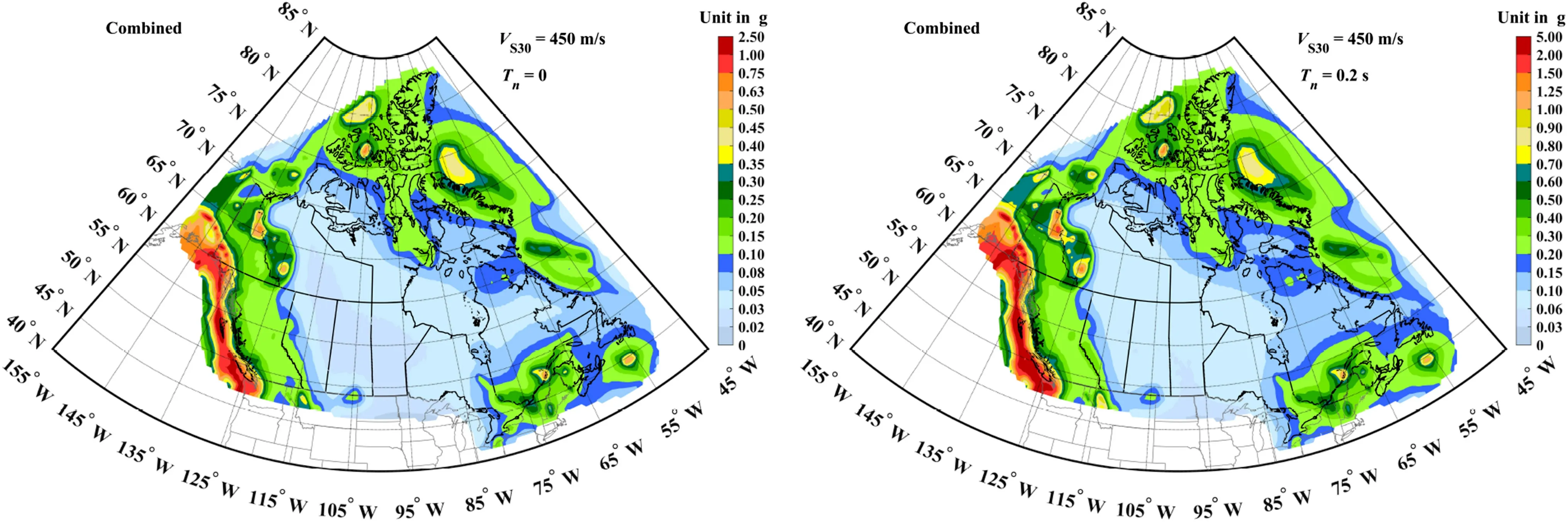
Fig.14 Seismic hazard map in terms of A 2475 and S 2475 (0.2) by considering the combined source model, that is, the combination of CanSSM6, f ixed kernel smoothing technique (FKSM), and adaptive kernel smoothing technique (AKSM) with weights equal to 0.5, 0.25,and 0.25, respectively

(3) In most cases, if the assessed intensities ofA Tand ST(T n) for a site using either source model are large,the obtained seismic hazards by using dif ferent source models tend to agree well.However, it is observed that the assessedA Tand ST(T n) for a site may be signif icantly large when using one model, while they can be comparatively small when another source model is utilized.

(4) The application of FKSM generally yields smoother seismic hazard contours compared to those obtained through the use of AKSM.

(5) On average, the use of CanSSM6 may underestimate the seismic hazard in comparison to the results obtained by using FKSM.However, the use of CanSSM6 can either underestimate or overestimate the seismic hazard relative to AKSM, depending on the specif ic vibration period considered.

(6) Given the absence of compelling justif ications to dismiss the spatially smoothed source models, it is suggested that multiple seismic source models can be considered as part of the logic tree for seismic hazard assessment.An example of such a combined source model, which assigns weights of 0.5 to CanSSM6,0.25 to FKSM, and 0.25 to AKSM, is employed to map the seismic hazard.On average, the results obtained by using CanSSM6 and the combined source models become relatively consistent.It must be emphasized that this consistency, which is based on average behavior, should not be extended to an individual site.

AcknowledgmentsThe support of the Fundamental Research Funds from the Central Universities, CHD (Grant No.300102282103),Natural Science Basic Research Program of Shaanxi (Program No.2023-JC-QN-0512), and Harbin Institute of Technology (Shenzhen),is gratefully acknowledged.

Open AccessThis article is licensed under a Creative Commons Attribution 4.0 International License, which permits use, sharing, adaptation, distribution and reproduction in any medium or format, as long as you give appropriate credit to the original author(s) and the source,provide a link to the Creative Commons licence, and indicate if changes were made.The images or other third party material in this article are included in the article's Creative Commons licence, unless indicated otherwise in a credit line to the material.If material is not included in the article's Creative Commons licence and your intended use is not permitted by statutory regulation or exceeds the permitted use, you will need to obtain permission directly from the copyright holder.To view a copy of this licence, visit http:// creat iveco mmons.org/ licen ses/ by/4.0/.