
Progress and future prospects of decadal prediction and data assimilation:A review
2024-03-04 07:25WnZhouJinxioLiZixingYnZiliShnBoWuBinWngRonghuZhngZhijinLi
Wn Zhou , , , Jinxio Li , , Zixing Yn , , Zili Shn , Bo Wu , Bin Wng , Ronghu Zhng ,Zhijin Li ,
a Key Laboratory of Polar Atmosphere-ocean-ice System for Weather and Climate of the MOE, Department of Atmospheric and Oceanic Science & Institute of Atmospheric Science, Fudan University, Shanghai, China
b Key Laboratory for Polar Science of the MNR, Polar Research Institute of China, Shanghai, China
c Shanghai Investigation, Design and Research Institute Co., Ltd., Shanghai, China
d LASG, Institute of Atmospheric Physics, Chinese Academy of Sciences, Beijing, China
e School of Marine Science, Nanjing University of Information Science & Technology, Nanjing, China
Keywords:
ABSTRACT Decadal prediction, also known as “near-term climate prediction ”, aims to forecast climate changes in the next 1–10 years and is a new focus in the fields of climate prediction and climate change research.It lies between seasonal-to-interannual predictions and long-term climate change projections, combining the aspects of both the initial value problem and external forcing problem.The core technique in decadal prediction lies in the accuracy and efficiency of the assimilation methods used to initialize the model, which aims to provide the model with accurate initial conditions that incorporate observed internal climate variabilities.The initialization of decadal predictions often involves assimilating oceanic observations within a coupled framework, in which the observed signals are transmitted through the coupled processes to other components such as the atmosphere and sea ice.However, recent studies have increasingly focused on exploring coupled data assimilation (CDA) in coupled ocean–atmosphere models, based on which it has been suggested that CDA has the potential to significantly enhance the skill of decadal predictions.This paper provides a comprehensive review of the research status in three aspects of this field: initialization methods, the predictability and prediction skill for decadal climate prediction, and the future development and challenges for decadal prediction.
1.Introduction
The slowdown in the rate of global surface warming during the early 2000s, and its regional variations, emphasized the significant role of decadal climate variability (DCV) in influencing long-term warming trends in the face of ongoing anthropogenic forcings (as discussed by Medhaug et al.(2017) ).This event, commonly referred to as a “pause ”or “hiatus ”in global warming, gained attention both in scientific circles and the public domain (as discussed by Lewandowsky et al.(2016) ).Scientists argued that this phenomenon was associated with longrecognized multiyear phenomena, particularly the oscillations of the ocean–atmosphere system in the tropical Pacific, which had been previously identified and assessed ( IPCC, 1996 ).
Kosaka and Xie (2013) indicated that the hiatus in global warming could be attributed to natural climate variability, particularly a La Ni?a-like decadal cooling in the eastern equatorial Pacific.Meehl et al.(2016) employed a novel approach based on physical phenomena to quantify the contribution of the Interdecadal Pacific Oscillation (IPO) to multidecadal global mean surface temperature (GMST)trends.They found that the positive IPO phase contributed 71% and 75% to the rapid GMST rise during the time periods from 1910 to 1941 and 1971 to 1995, respectively, while the transition of the IPO from a positive to a negative phase in the late-1990s accounted for 27%of the temporary suppression of GMST rise.In addition, several studies have also proposed that volcanic aerosols played a role in the recent hiatus in global warming via changes in Earth’s energy balance at the top of the atmosphere ( Humber and Knutti, 2014 ; Santer et al.,2017 ).
Indeed, the oceans play a central role in DCV, due to their thermal and dynamical inertia, regardless of whether the forcing is external (such as from solar variations or volcanic activity) or internal (from interactions within the climate system).Changes in ocean heat content can impact the exchange of heat with the atmosphere, affecting surface temperatures and atmospheric circulation patterns ( Sutton and Hodson, 2005 ; Mantua et al., 1997 ; Li and Bates, 2007 ; Mochizuki et al.,2010 ).The decadal oscillations in the Pacific Ocean and Atlantic Ocean can have significant impacts on the climate of adjacent regions, affecting the lives and property of people in neighboring countries.A typical example is the significant weakening of the East Asian summer monsoon in the late 1970s ( Ding et al., 2008 ).This weakening is characterized by a decrease in the low-level (850 hPa) southwestly winds and an enhancement of the upper-level (200 hPa) westerly jet south of its normal position ( Yu and Zhou, 2007 ).As a result, there has been increased rainfall in the Yangtze River basin and decreased rainfall in northern China, which has caused numerous casualties and significant economic losses ( Huang and Zhou, 2002 ).Li et al.(2006) also pointed out that decadal fluctuations in sea surface temperature (SST) over the southern Indian Ocean also play a significant role in the Asian summer monsoon.Therefore, climate change at decadal timescales and its impacts on economic and social development have attracted widespread attention in society.Due to its significant scientific value as a crucial reference for national medium- to long-term decision-making, it has gradually gained attention from the international scientific community ( Meehl et al.,2009 ; Hurrell et al., 2009 ).This motivates the ongoing development of “initialized decadal prediction ”, a method that involves initializing coupled models with observed ocean conditions while prescribing anthropogenic and natural forcings.These models are then run for multiple years with the aim of predicting the combined effects of radiative forcing and natural climate variability since the 1960s ( Kirtman et al.,2013 ).
Decadal prediction, also known as “near-term climate prediction ”,focuses on forecasting climate changes for the next 1–10 years.The study of decadal prediction started relatively late and gradually became an important and challenging scientific issue in the field of climate change in the late 1990s.The World Climate Research Program established the Climate Variability and Predictability program in 1995,which included decadal-scale climate variability, climate change, and predictability as important research topics.Decadal prediction falls between seasonal-to-interannual prediction and long-term climate change prediction ( Troccoli and Palmer, 2007 ; Osman et al., 2023 ).Phase 5 of the Coupled Model Intercomparison Project (CMIP5) included decadal prediction experiments as one of the core experiments for climate change simulations for the first time ( Taylor et al., 2012).The other core experiment focused on century-scale long-term climate simulations and projections.The current phase of CMIP (i.e., CMIP6) includes decadal predictions as one of its subprojects, known as the Decadal Climate Prediction Project ( Eyring et al., 2016 ).
At decadal time scales, the potential prediction skill primarily arises from three factors: changes in external forcing, the inertia of the climate system, and decadal oscillations driven by internal variability( Meehl et al., 2009 ).External forcing in the climate system includes natural forcing such as solar activity and volcanic eruptions, as well as human-induced greenhouse gas and aerosol emissions.At the 1–10 year timescale, the influence of internal variability is comparable to, or even greater than, external forcing ( Meehl et al., 2009 ).Therefore, decadal predictions require both the initialization of models to capture the internal variability of the climate system and the consideration of radiative external forcing (including human activities and natural forcings)( Taylor et al., 2012 ).Initialization serves two purposes: firstly, it allows the internal variability (such as Pacific Decadal Oscillation (PDO) and Atlantic Multidecadal Oscillation (AMO)) of models to be synchronized with the observations as closely as possible in terms of phase and intensity.Secondly, it can correct biases in models’ responses to greenhouse gas forcing ( Smith et al., 2013 ).Therefore, initialization is crucial for the success of decadal predictions.Currently, the level of decadal prediction worldwide is still in its early stages, and factors influencing its accuracy include the performance of the initialization method, the performances of models, and the quality of observational data ( Taylor et al.,2012; Zhou and Wu, 2017 ).While continuously improving the performances of models and enhancing the quality of observations, it is crucial and indispensable to improve the quality of initial conditions through advanced initialization methods.This is an urgent task in decadal prediction and a key component for improving its accuracy.
2.Assimilation methods applicable to coupled climate system models
Data assimilation (DA) algorithms need to be integrated with coupled ocean–atmosphere general circulation models (CGCMs) to form an assimilation system.However, DA algorithms for CGCM initialization can be classified into two types: coupled and uncoupled.For uncoupled DA methods, the assimilation system uses atmosphere and ocean model forecast results as the first guesses.The calculation process does not take into account the coupling between the atmosphere and ocean models.For coupled DA methods, the first guesses are calculated by the entire coupled model.The assimilation algorithms used in uncoupled DA and coupled DA are similar ( Fig.1 ).
2.1.Nudging
Nudging is one of the earliest methods used in atmospheric DA( Hoke and Anthes, 1976 ).Its principle involves adding a forcing term to the set of numerical model dynamic forecast equations.The formula for nudging can be represented as
wherexrepresents the model forecast variable,trepresents the time,F(x) represents the original forecast of models,xobsrepresents the observed variable,αis the nudging coefficient, andα(xobs -x) is the observational forcing term.The advantage of the nudging algorithm is that its formula is simple with clear physical meaning.It is easy to implement in models and has a low computational cost.The drawback of the nudging algorithm is that the strength coefficient that approaches the observation requires manual adjustment.It is closely related to factors like the model integration step length, and simultaneous assimilation of multiple variables can easily cause instability in model integration.Many modeling centers have used the nudging method when conducting seasonal to interdecadal forecasts with climate system models.
Chen and Lin (2013) used the nudging and time-lag perturbation methods to establish an ensemble initialization system and carried out tropical cyclone (TC) seasonal forecasts.Hudson et al.(2017) established a new Bureau of Meteorology prediction system named ACCESSS1 by using the nudging method.Xin et al.(2018) used the nudging method as the initialization scheme for BCC_CSM1.1, and carried out decadal predictions.The results showed a significant improvement in the skill for summer surface temperature prediction in eastern China compared to the previous version.

Fig.1.Schematic of (a) uncoupled DA and (b) coupled DA (modified from Fig.1 in Zhang et al.(2020) ).
2.2.Variational DA
2.2.1.Three-dimensionalvariationalDA
The mathematical essence of three-dimensional variational DA(3DVar) is to find the optimal solution to minimize the cost function( Parrish and Derbber, 1992 ), which is consistent with the purpose of optimum interpolation (OI) analysis.3DVar inherits the advantages of OI and improves computational efficiency.Courtier et al.(1998) replaced ECMWF’s assimilation method from OI to 3DVar and found that 3DVar could fully inherit the characteristics of OI and handle small-scale noise more effectively.
The mathematical expression for the objective function can be represented as
wherexb represents the background field of the model,Bis the covariance matrix of the model background error,yobsstands for the observation,His the observation operator, andRis the covariance matrix of the observation error.The optimal analysis initial value (in the case whenin Eq.(2) ) can be represented as
The advantage of 3Dvar is that it considers the global threedimensional space when solving the cost function, and all observation data can be used simultaneously.Besides, 3DVar only changes the initial value of the model and does not alter the integration process of the model.Du et al.(2012) used 3DVar as the ocean initialization scheme for a coupled atmosphere–ocean model named EC-Earth and conducted decadal predictions.The results indicated that the ocean assimilation algorithm improved the prediction skill for sea-ice area and ocean heat content.Zang et al.(2022) optimized the 3DVar algorithm for handling multiscale information (especially small-scale), which enhanced the applicability of the 3DVar algorithm in weather–climate integrated modeling.
2.2.2.Four-dimensionalvariationalDA
Four-dimensional variational DA (4DVar) considers the dimension of time when seeking the optimal solution for the cost function, and can be understood as an upgraded version of 3DVar.The approach of 4DVar defines a time window, considering the evolution of data within this time frame.Assuming that there arent+1observations withinnttime moments, the mathematical expression for the objective function can be represented as
whereHjrepresents the observation operator at momentj;Mt0→tjrepresents the integration from momentt0to momenttjthrough a nonlinear model; andyjobs ,HjMt0→tjx, andRjrepresent the observation, the model-simulated observation, and the observation error covariance matrix at momentj.The optimal analysis initial value (in the case whenin Eq.(4) ) can be represented as

2.3.Incremental analysis updates
Bloom et al.(1996) first proposed the Incremental Analysis Updates(IAU) assimilation method.This method, similar to the nudging assimilation method, involves adding an observational recovery forcing term to the set of model dynamic forecast equations.The formula for nudging can be represented as
where Δxarepresentsthe analysis increment at the midpoint ofthe assimilationwindow,τrepresents thelength of thewindow, andΔxais the observational forcing term.The difference between IAU and nudging is that the observational forcing term does not change within the time window.This makes the model more stable during integration, but IAU requires more computational resources.In current prediction systems, IAU is widely applied as a forecasting procedure, often used in combination with methods such as variational DA ( Lee et al., 2006b ;Shimose et al., 2017 ) and OI ( Sun et al., 2018 ).Li et al.(2021b) established a prediction system based on FGOALS-f2 that is suitable for subseasonal-to-interdecadal forecasts by adopting the IAU assimilation method and time-lagged ensemble perturbation method.FGOALS-f2 shows considerable skill in predicting global TC activity, the propagation of Madden–Julian Oscillation, and El Ni?o–Southern Oscillation(ENSO).Tatebe et al.(2012) established an initialization module for the various versions of MIROC, based on the IAU coupled assimilation algorithm, and carried out decadal predictions.The results showed that the latest version of MIROC offered a significant improvement in the decadal prediction skill for SST and corresponding modes in the North Atlantic, the subtropical North Pacific, and the Indian Ocean.
2.4.Ensemble perturbation DA method
Unlike the methods introduced previously, the ensemble perturbation assimilation method uses a large ensemble sample to estimate the background error covariance matrix.In principle, ensemble perturbation assimilation can be divided into dynamic perturbation and static perturbation methods.The dynamic ensemble perturbation method refers to the fact that the background error covariance matrix will undergo local or global dynamic adjustments as the model integrates.The Ensemble Kalman Filter (EnKF) and Ensemble Adjustment Kalman Filter(EAKF) are two representative dynamic ensemble perturbation assimilation methods.In order to implement Bayes’ Theorem, the EnKF method dynamically estimates the background covariance matrix by generating a considerable number of ensemble samples, and research has found that it facilitates multi-cycle layer coupled assimilation.The disadvantage of the EnKF approach is that, under the conditions of limited ensemble samples, it faces the problem of under-sampling and requires localization and inflation.This increases the computational overhead.The EAKF method is a variant of the EnKF method under an adjustment idea, as it requires fewer ensemble samples to estimate the background covariance matrix, it is suitable for conducting decadal predictions with CGCMs.Li et al.(2018) developed an ensemble prediction system based on the Coupled Model, version 2.1, and the EAKF method, and the results indicated that the prediction system is capable of capturing the regime transition of the Atlantic Meridional Overturning Circulation (AMOC)( Liu et al., 2021 ).Pohlmann et al.(2023) developed an assimilation scheme based on ICON-ESM (Icosahedral Non-hydrostatic Earth System Model) and found the prediction skill was improved in regions of the tropical Pacific.
Besides, some simplified ensemble assimilation methods have also been applied to weather–climate predictions.Li et al.(2021b) developed a coupled seamless prediction system with FGOALS-f2 based on nudging and IAU operators.Using 24 ensemble reanalysis experiments,the results showed that the model exhibited considerable prediction skill for ENSO and TCs.The Seamless System for Prediction and Earth System Research at the Geophysical Fluid Dynamics Laboratory of the National Oceanic and Atmospheric Administration utilizes the nudging method in the atmospheric, land surface, and sea ice components; while in the ocean component, it utilizes the EAKF method ( Lu et al., 2020 ;Delworth et al., 2020 ).Wu et al.(2018) developed a coupled assimilation method called EnOI-IAU, which is applicable for interdecadal prediction.EnOI-IAU integrates the features of Ensemble Optimal Interpolation (EnOI) and IAU.Specifically, the former’s background error covariance matrix is derived from a static historical ensemble, and it gradually incorporates analysis increments into models over time through constant forcing terms in prognostic equations.Hu et al.(2020) found that IAP-DecPreS, based on EnOI-IAU and FGOALS-s2, has considerable predictive skill for ENSO.Lu et al.(2023) developed a multi-timescale high-efficiency approximate filter with EnOI (MSHea-EnOI) scheme and found that MSHean-EnOI has the potential to improve the prediction skill with increased representativeness on multiscale properties.
2.5.Hybrid DA methods
To incorporate the characteristics of different types of assimilation operators, hybrid assimilation operators have become a research hotspot.Currently, the primary focus is on operators that combine ensemble perturbations with variational methods.Hamill and Snyder (2000) were the first to combine the features of 3DVar and EnKF,resulting in the development of the En3Dvar operator.Unlike the traditional 3DVar algorithm, the estimation of background error covariances in En3Dvar originates from two parts:
One part is the covariance matrixPbcalculated from ensemble samples, and the other part is the 3DVar background error covariance matrixVbthat has undergone weight optimizationβ.Similarly, many studies also combine ensemble perturbations with 4DVar ( Tian and Feng, 2015 ;Zhang et al., 2009 ; Johnson et al., 2005 ; Shi et al., 2023 ).Considering the characteristic of 4DVar requiring substantial computational resources, Wang et al.(2010) developed an economical approach to conducting 4DVar computations based on the dimension reduced projection(DRP) method.He et al.(2017) established a CDA system based on DRP-4DVar and the climate system model FGOALS-g2 for decadal climate predictions, which can separately assimilate observations or reanalysis products from the ocean ( He et al., 2020b ), atmosphere ( Li et al.,2021a ), and land surface ( Shi et al., 2022 ).Tian and Feng (2019) developed a hybrid DA method called CNOP–4DVar, which takes the advantages of both the conditional nonlinear optimal perturbation (CNOP)( Mu et al., 2003 ) and 4DVar methods.
2.6.Integrating artificial intelligence algorithms with DA
Machine learning (ML), particularly deep learning (DL) algorithms,have achieved remarkable results in fields such as image recognition,classification, and natural language learning, in line with the rapid development of computer technology.In the field of meteorology, weather forecasting systems based on artificial intelligence (AI) models have already surpassed traditional numerical prediction models in some performance indicators for nowcasting ( Ravuri et al., 2021 ), medium-range weather forecasting ( Bi et al., 2022 ; Lam et al., 2022 ), and climate prediction ( Ham et al., 2019 ).In fact, ML and DA share many similarities:(1) They are both used as “inverse methods ”to learn about the world from data, which can be united under a Bayesian framework.(2) Both ML and variational DA usually employ gradient descent techniques to minimize the cost or loss function.The cost function in variational DA is equivalent to the loss function for training a neural network.Recently,many studies have attempted to combine ML and DA.
Arcucci et al.(2021) developed a Deep Data Assimilation (DDA) operator, a method that integrates DA with ML.Their results indicated that DDA shows great capability in approximating nonlinear systems,and extracting high-dimensional features, which is difficult to overcome for DA algorithms.Tsuyuki and Tamura (2022) embedded deep neural networks (DNNs) into EnKF, developing a Deep Learning-EnKF (DLEnKF) algorithm.Compared to EnKF, DL-EnKF requires a smaller ensemble size to accurately estimate the background covariance matrix.Dong et al.(2022) developed a pure data-driven 4DVar implementation framework named ML-4DVAR, based on the bilinear neural network method, and the results indicated that the ML-4DVAR framework can achieve better assimilation results and significantly improve computational efficiency.

Fig.2.Schematic of assimilation methods for different forecasting and prediction timescales.
In summary, different DA methods and strategies are suitable for different forecast durations ( Fig.2 ).Uncoupled DA is primarily used for short-term to seasonal-scale forecasts, while longer-term forecasts generally require consideration of multi-component coordination.Therefore, most DA methods for interannual to decadal predictions are coupled.For short-term and mid-term forecasts, assimilation methods are often more “complex ”, and variational assimilation, ensemble perturbation, and other methods are widely used in this time period.For medium to long-term climate prediction, it is necessary to consider the overall computational efficiency of the forecasting system, so “simpler ”assimilation methods are preferred, and the coordination of initialization in different component needs to be considered.
3.Predictability and prediction skill for decadal climate prediction
Decadal-scale climate anomalies are influenced by both initial-value issues and external forcing boundary conditions ( Meehl et al., 2009 ;Kushnir et al., 2019 ).Therefore, decadal climate prediction can be regarded as a combination of the initial-value problem linked to the internal variability of the climate system and the external-forcing problem( Fig.3 ).

Fig.3.Contributions of initial conditions and external forcing in seamless prediction ( Fig.1 in Boer et al.(2016) ).
At the decadal scale, the prediction skill for climate anomalies is mainly determined by three factors: changes in external forcing, the thermal inertia of the climate system, and decadal oscillations caused by internal variability of the climate system ( Meehl et al., 2009 ).External forcing includes both natural forcing (solar activity, volcanic eruptions, etc.) and anthropogenic forcing (greenhouse gas emissions,aerosol emissions, ozone, land-use changes, etc.) ( Lee et al., 2006a ).The thermal inertia of the climate system is a result of the large heat capacity of the oceans and their stable stratification, leading to slow climate processes.For example, even if greenhouse gas concentrations remain at current levels, the global average surface temperature is projected to continue increasing at a rate of 0.1°C/10 yr over the next few decades,resulting in a warming of approximately 0.6°C by 2100 ( Meehl et al.,2005 ).The internal decadal variability signals in the climate system mainly include the PDO, AMO, and others.
Currently, apart from improving model performance and enhancing the quality of observational data, the development of accurate and reasonable model initialization schemes is a key factor influencing the skill of decadal predictions ( Taylor et al., 2012 ).Currently, the initialization schemes of international decadal prediction systems mainly focus on ocean initialization.However, studies have indicated that besides ocean initialization, the initialization of other subsystems of the climate system may also affect decadal prediction skill ( Merryfield et al., 2013 ;Saha et al., 2010 ; Bellucci et al., 2015 ).Climate anomaly signals within these subsystems propagate through multi-layer interactions in the climate system, thus influencing the entire climate system.However, due to the smaller heat capacity of these subsystems compared to the oceans,their contributions to decadal variability and predictability are still uncertain.In addition, the limited understanding of the physical processes involved in these subsystems, the need for improvement in modeling their dynamics, and the lack of reliable observational data for initialization have resulted in fewer models incorporating initialization for these subsystems.
3.1.Prediction skill of current decadal climate prediction experiments
The prediction skill of decadal prediction experiments mainly depends on the modeling capability, accuracy of initial conditions, and external forcing ( Boer et al., 2016 ; Kirtman et al., 2013 ).Compared to historical climate simulations and climate projections without initialization, initialized decadal prediction experiments have shown significant improvements in predicting the global mean temperature, the mid-1970s decadal phase transition of Pacific SST, the mid-1990s decadal phase transition of the North Atlantic, and the early 21st-century global warming hiatus ( Doblas-Reyes et al., 2013 ; Guemas et al., 2013a ;Keenlyside et al., 2008 ; Kirtman et al., 2013 ; Meehl et al., 2014, 2021 ;Meehl and Teng, 2014 ; Mochizuki et al., 2010 ; Smith et al., 2007 ).The prediction skill of decadal prediction experiments primarily originates from the low-frequency variations of SSTs, such as ENSO, the PDO,and AMO ( Meehl et al., 2021 ).The following subsections discuss the prediction skill of decadal prediction experiments for SST in different ocean basins.
3.2.1.PacificOcean
The Pacific Ocean plays a significant role in shaping climate anomalies in East Asia, both on interannual and decadal scales (for example,both ENSO and the PDO are low-frequency signals over the Pacific, and have noteworthy impacts on climate variability in East Asia).However,the current decadal prediction skill for the Pacific in many models is generally limited ( Fig.4 ).Numerous studies have emphasized the pressing societal demand for, and scientific importance of, improving the prediction of ENSO several years ahead ( Petrova et al., 2020 ; Chen et al.,2004 ; Luo et al., 2008 , 2017 ; Chikamoto et al., 2015 ).Advanced dynamical models have achieved high prediction skill for ENSO, accurately forecasting it up to 12 months in advance ( Barnston et al., 2019 ).Additionally, Ham et al.(2019) indicated that ML techniques can enhance ENSO predictions up to 18 months ahead, surpassing the predictive skill of dynamical models.
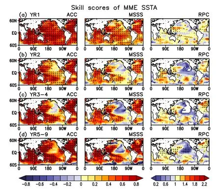
Fig.4.Prediction skill for SSTAs: (a) anomaly correlation coefficient (ACC), mean square skill score (MSSS), and ratio of predictable components (RPC) for multimodel ensemble mean (5 CMIP5 models and 10 CMIP6 models) SSTA predictions at a 1-year lead time.The 95% confidence level is signified by the black dotted areas.(b–d) As in (a) but for the prediction skill at lead times of 2 years, 3–4 years, and 5–9 years, respectively (Fig.1 in Choi and Son (2022) ).
Mochizuki et al.(2010) showed that MIROC exhibits significant prediction skill for the PDO, based on the IAU assimilation scheme.Lienert and Doblas-Reyes (2013) found that the significant prediction skill for the PDO is at 1–2-year lead time by using the DePreSys decadal prediction system from the Hadley Centre.Wu et al.(2018) , utilizing the EnOI-IAU initialization scheme, reported correlation coefficients exceeding 0.9 between the observed and initialized SST anomalies (SSTAs)in the equatorial central-eastern Pacific, and coefficients above 0.7 for the North Pacific (the key region for the PDO).Recently, Choi and Son (2022) suggested that current climate models can forecast ENSO one year in advance, while longer lead-time predictions for winter ENSO require larger ensemble sizes.Moreover, significant prediction skill for the PDO can be achieved at lead times of 5–9 years, primarily driven by models’ responses to external forcing rather than initialization effects (with the latter only persisting for two years).Recently,He et al.(2023) achieved significant prediction skill for the PDO at lead times from 1 to 10 years, as well as in the 10-year mean, which is higher than the skills of most CMIP5 and CMIP6 hindcasts.This high prediction skill for the PDO is mainly attributable to the DRP-4DVar-based initialization using air–sea interactions as a constraint ( He et al., 2023),consistent with the consensus that the PDO is the product of air–sea interactions.
3.2.2.IndianOcean
The Indian Ocean has emerged as a region in which models exhibit relatively high decadal prediction skill globally, primarily due to the influence of radiative external forcing ( Van Oldenborgh et al.,2012 ; Ho et al., 2013 ; Wu et al., 2018 ).This can be attributed to the pronounced impact of external forcing resulting from greenhouse gas increases, surpassing the influence of internal variability.Consequently, the contribution of internal variability to decadal changes in Indian Ocean SST is relatively minor ( Guemas et al., 2013b ; Dong and Zhou, 2014 ; Dong et al., 2014 ).Dong et al.(2016) emphasized the predominant influence of the PDO on the decadal variability observed in the Indian Ocean.Moreover, it has been suggested that decadal variations in Indian Ocean SST can exert modulation on the interannual variability in the Indian Ocean–Pacific region ( Meehl and Arblaster, 2011 , 2012 ).Therefore, by refining the initialization scheme for the Indian Ocean, the prediction skill for certain interannual variations in the Asian–Australian monsoon region can be significantly enhanced.Kim et al.(2012) utilized coupled GCMs and demonstrated that the ensemble mean of these models exhibited higher prediction skill for Indian Ocean SST at 2–5- and 6–9-year lead times.Wu et al.(2018) highlighted that the Indian Ocean consistently exhibits superior prediction skill for annual mean SST in hindcast years 2–5 and 6–9, with correlation coeffi-cients surpassing 0.8 when compared to observations based on decadal prediction experiments utilizing FGOALS-s2 and the EnOI-IAU initialization scheme.However, it should be noted that significant positive correlations for detrended SST anomalies are observed only in specific areas of the southern Indian Ocean.
3.2.3.AtlanticOcean
Previous studies have indicated that initialized decadal prediction experiments significantly enhance the prediction skill for North Atlantic SST ( Van Oldenborgh et al., 2012 ; Doblas-Reyes et al., 2013 ;Meehl et al., 2014 ; Robson et al., 2014 ; García-Serrano et al., 2015 ).This improvement is likely associated with the initialization process incorporating the initial state of AMOC ( Delworth et al., 2007 ; Knight et al.,2005 ; Swingedouw et al., 2012 ).Previous research has also emphasized that accurate initialization of AMOC is crucial for achieving better prediction skill for North Atlantic SST and upper-ocean heat content compared to persistence forecasts up to a decade in advance ( Latif and Keenlyside, 2011 ; Yeager et al., 2012 ; Meehl et al., 2014 ).
Ho et al.(2013) distinguished the impacts of external forcing and initial conditions on Atlantic SST based on a statistical model, and indicated that the prediction skill for midlatitude Atlantic SST was primarily influenced by external forcing, whereas the prediction skill for North Atlantic and South Atlantic SST was mainly driven by the initial conditions.Wu et al.(2015) further suggested that the enhanced prediction skill for North Atlantic SST is partially attributable to the improved prediction skill for the AMO through initialization.Additionally, different climate system models employing the same IAU initialization scheme exhibit varying prediction skills in the Atlantic region, underscoring the influence of model performance on decadal prediction skill.
4.Advancing the study of decadal prediction
4.1.Use of AI techniques
Using the state-of-the-art 4DVar approach ( Bauer et al., 2015 ;Huang et al., 2009 ; Mochizuki et al., 2016 ), DA into climate models is expensive in terms of both human development effort and computing power.AI techniques are indispensable for making sense of the exponentially growing amount of data and addressing the increasingly complex requirements in weather forecasting, climate monitoring, and decadal prediction.For example, a convolutional neural network was successfully employed to accurately predict ENSO events with lead times of up to one and a half years, surpassing the skill of dynamical physical forecast models ( Ham et al., 2019 ).However, a challenge in training decadal climate prediction models is the limited availability of observational data for proper training.
4.2.Applications of statistical methods
Some researchers have also attempted to predict future decadal climate states using purely statistical methods based on time series decomposition techniques.For example, Empirical Mode Decomposition(EMD), a widely used technique in engineering, has been extended to the field of climate change research.Many scholars have started employing EMD to decompose long-term observed temperature series at global, regional, or representative stations, extracting their trends and decadal variations.Subsequently, regression equations are established using these components to forecast temperature changes for the coming decades ( Fu et al., 2011 ; Qi et al., 2017; Wei et al., 2015 ; Wu et al.,2015 ).Wu et al.(2019) developed a practical dynamical–statistical combined approach for decadal prediction and found that the prediction skill for surface air temperature over land in summer in the Northern Hemisphere was significantly improved.Additionally, empirical approaches that make use of observed teleconnections between the ocean and land should be promoted, as they can provide valuable insights ( Lean and Rind, 2009 ; Suckling et al., 2017 ).
4.3.Model drift reduction
Reducing model biases and drift is also a promising approach, as these systematic errors can negatively impact the spatial representation and temporal variability of DCV patterns.In forecast mode, model drift occurs when models initialized from observed conditions gradually adjust toward their own biased equilibria.It is important to identify the physical origins of model drift and systematic errors, as understanding these mechanisms can provide insights into the underlying processes of DCV in models.This knowledge can then be used to improve the simulation and prediction capability/skill of DCV.Promoting research in this area is a promising pathway for advancing the understanding and prediction of DCV ( Toniazzo and Woolnough, 2014 ; Sanchez-Gomez et al.,2016 ; Zhang et al., 2018 ).He et al.(2017) indicated that an advanced initialization scheme was able to significantly reduce this initial drift in decadal climate prediction.Therefore, developing or applying sophisticated DA approaches to initialize decadal climate predictions may assist in restricting initial model drift.
4.4.Improving knowledge on the energy balance of Earth’s climate system
Enhancing our understanding of the mechanisms governing climate variability and change at decadal time scales requires a concerted effort to improve knowledge and observational capabilities in tracking energy flows through the climate system.Advances in satellite technology, including satellite-based measurements of key climate variables such as SST, ocean heat content, and atmospheric circulation patterns, have greatly enhanced our ability to monitor and analyze the energy balance of Earth’s climate system.Additionally, the development of advanced DA techniques, which combine observations with climate models, has improved our ability to estimate and predict changes in the energy flows within the system.
One key area of focus is the quantification of the energy exchange between the atmosphere and the ocean.This involves studying the processes governing the transfer of heat, moisture, and momentum between these two components of the climate system.Understanding these exchanges is crucial for predicting regional climate variations, as the ocean plays a significant role in modulating atmospheric circulation patterns and influencing weather patterns on various time scales.
Another important aspect is the investigation of energy transport and storage within the climate system.This involves studying the role of ocean currents, atmospheric circulation patterns, and other dynamic processes in redistributing energy across different regions of the Earth.Advances in ocean observing systems, such as the deployment of Argo floats and enhanced measurements from research vessels, have provided valuable data for studying these energy transport processes.
Furthermore, efforts to improve the representation of cloud processes in climate models are crucial for accurately simulating the energy balance of the climate system.Clouds play a critical role in regulating the amount of incoming solar radiation that reaches Earth’s surface and the amount of outgoing infrared radiation that escapes into space.Improving our understanding of cloud formation, evolution, and their interactions with other components of the climate system is essential for reducing uncertainties in decadal climate predictions.
4.5.Mining of paleoclimate proxy data
In order to enhance our understanding of DCV, it is valuable to combine the analysis of instrumental observations and models with highresolution paleoclimate proxy data.Paleoclimatic archives can provide evidence of coherent spatial and temporal patterns of DCV ( Linsley et al.,2015 ; Tierney et al., 2015 ; Emile-Geay et al., 2017 ; Reynolds et al.,2017 ).These data sources can provide valuable insights into the fundamental physical processes driving DCV and can serve as a validation tool for patterns identified in the relatively short instrumental record.Furthermore, efforts to rescue and digitize instrumental data should be expanded, the aiming being to recover undigitized records and increase overlap with paleoclimatic archives.
4.6.Considering the multivariate nature of DCV
A reconsideration of the conventional definition of DCV phenomena is necessary.It is important to exercise caution when representing and interpreting the climate system using single univariate and basin-wide indices, which is often the case with the AMO and IPO indices (refer to examples in Yeager and Robson (2017) ).It is recommended that the scientific community use acronyms for decadal variability (e.g., AMV and IPV) to facilitate thinking in terms of broad spectrum variability rather than temporal oscillations with specific time scales.These recommendations aim to enhance our understanding and description of DCV phenomena.
Efforts in collecting, analyzing, and interpreting high-resolution climate records play a crucial role in understanding decadal-scale teleconnections between the tropics and midlatitudes, as well as inter-basin interactions ( An et al., 2021 ).Developing spatiotemporal reconstructions of climate variability, particularly for the past two millennia, can enhance our knowledge of tropical–extratropical teleconnections.Recent studies have emphasized the impact of mesoscale oceanic fronts on atmospheric dynamics and the crucial role played by the stratosphere and storm tracks in transmitting variations in SST to the continents.To advance this further, allocating adequate computing resources to generate large ensembles is essential for accurately capturing internal variability,attributing observed decadal climate variations, understanding their nature and physical origins, and investigating their interactions with external forcing.
5.Conclusion and prospects
A comprehensive review of initialization methods, the current status of decadal prediction, and new theories and technologies for improving prediction skills is provided in this paper.Despite significant achievements having been made in DCV and predictability (DCVP), certain challenges and issues still remain, including:
(1) Improving models’ abilities to simulate and predict decadal variability: It is necessary to correct any inaccuracies or systematic errors in models’ portrayals of climatologies.Efforts should be made to improve models’ performances in simulating decadal variations, considering factors such as the spatial and temporal scale, as well as the low signal-to-noise ratio.The resolution of climate models also plays a critical role in decadal prediction accuracy ( Monerie et al., 2017 ;Sun et al., 2022 ).Fine-scale resolution enhances the model’s ability to capture important oceanic and atmospheric interactions, such as ocean currents, heat transport, and teleconnections, which are crucial for accurate decadal predictions.It also requires enhancing the model’s capability to distinguish and capture meaningful decadal signals amidst background noise.For example, Lin et al.(2019) successfully simulated two time periods of the AMO by improving model performance, which contributed to understanding the connection between the atmosphere and oceans across different basins at decadal scales.When incorporating observed data, it is important to minimize sudden shifts or gradual deviations in the model’s initial conditions.Techniques need to be developed to assimilate real-world observations effectively, reducing discrepancies and ensuring a smoother transition between model state.The inclusion of external factors, such as aerosols, natural and human-induced influences, is crucial.It is necessary to understand and simulate the complex interactions between these agents and the atmospheric circulation and clouds.Examples include studying how aerosols interact with cloud formation and investigating the intricate relationships between ozone and radiation in the stratosphere.
(2) Advancing understanding of the mechanisms of DCV: Investigating the influence of external factors, such as solar variability and volcanic eruptions, on DCV is important.Understanding their mechanisms and impact on predictability and prediction can enhance our ability to account for these factors in models and improve the accuracy of decadal forecasts.Decadal climate signals can be relatively weak compared to background noise, making accurate prediction challenging, meaning developing methods to effectively extract and separate meaningful decadal signals from noise in both land and atmospheric predictions is crucial.While current models exhibit some skill in predicting decadal variations in the Atlantic region, the same level of predictability has not been achieved for the Pacific.Understanding the reasons behind this discrepancy and addressing the obstacles to predicting Pacific decadal variability are also important.In addition, investigating the origins, roles and mechanisms of interactions between different ocean basins on decadal timescales is essential.Examining how decadal climate anomalies may change in a warmer climate is crucial for understanding future climate projections.Additionally, understanding how volcanic eruptions’ impacts depend on the background state is important.Addressing the challenge of mean-state dependence, where the background climate conditions affect decadal variability, requires improved modeling and analysis techniques to accurately capture and incorporate these influences in predictions.
(3) Overcoming data-related challenges in DCVP: Utilizing paleoclimate data (particularly incorporating high-resolution proxies from the Common Era) in DCVP models can improve our understanding of long-term climate dynamics and enhance prediction capabilities.Employing a prediction ensemble, which consist of multiple models run with slightly different initial conditions or model parameters, can help us better understand decadal mechanisms.Ensembles provide a range of possible outcomes and enable us to assess the robustness and uncertainty of predictions, improving our confidence in the results.Enhancing our knowledge and data on natural and anthropogenic aerosols, as well as solar forcing, is crucial.These external factors play significant roles in decadal climate variability, and accurately quantifying their impacts requires comprehensive and reliable observational data.Improvements in data collection and analysis methods can lead to more accurate representation of external forcing agents in DCVP models.
(4) Overcoming the challenges in CDA: CDA is a promising approach that shows potential for enhancing weather and climate prediction.It offers several advantages over uncoupled DA methods: First, CDA can generate a more equitable state estimation for coupled prediction, ensuring that the model represents the interaction between different components of the Earth system accurately.Second, CDA can greatly improve the estimation of variables in sparsely sampled components, such as sea ice.Thirdly, CDA allows for the optimization of model parameters within the coupled framework and provides valuable insights into the interactions and feedbacks between different components of the coupled system.However, there are still challenges to overcome in CDA.For example, implementing a computationally efficient CDA algorithm in a high-resolution coupled model is a complex and challenging task that requires expertise in both DA and the specific coupled model framework; and considering the multi-scale information of models and observations is also challenging.Addressing these challenges requires multidisciplinary collaborations across various Earth science disciplines and advancements in computing algorithms.
Funding
This work was supported by the National Natural Science Foundation of China [Grant Nos.42192563 and 42120104001 ].
 Atmospheric and Oceanic Science Letters2024年1期
- Atmospheric and Oceanic Science Letters的其它文章
- Slowing down of the summer Southern Hemisphere Annular Mode trend against the background of ozone recovery
- Comparison between ozonesonde measurements and satellite retrievals over Beijing, China
- Decadal prediction skill for Eurasian surface air temperature in CMIP6 models
- Ascending phase of solar cycle 25 tilts the current El Ni?o–Southern oscillation transition
- The Tibetan Plateau bridge: Influence of remote teleconnections from extratropical and tropical forcings on climate anomalies
- Anthropogenic influence on the extreme drought in eastern China in 2022 and its future risk