
GLOBAL CLASSICAL SOLUTIONS OF SEMILINEAR WAVE EQUATIONS ON R3×T WITH CUBIC NONLINEARITIES*
2024-03-23 08:02陶飛
(陶飛)
School of Science, Nanjing University of Posts and Telecommunications, Nanjing 210023, China E-mail: 1458527731@qq.com
Abstract In this paper, we establish global classical solutions of semilinear wave equations with small compact supported initial data posed on the product space R3×T.The semilinear nonlinearity is assumed to be of the cubic form.The main ingredient here is the establishment of the L2-L∞decay estimates and the energy estimates for the linear problem, which are adapted to the wave equation on the product space.The proof is based on the Fourier mode decomposition of the solution with respect to the periodic direction, the scaling technique,and the combination of the decay estimates and the energy estimates.
Key words semilinear wave equation; product space; decay estimate; energy estimate;global solution
1 Introduction
The topic of the well-posedness of wave equations on product spaces arises from studying the propagation of waves along infinite homogeneous waveguides (see [14, 32, 35]) and the Kaluza-Klein theory (see [25, 29]).A natural feature of this topic is spatial anisotropy, which is different from the classical theory for hyperbolic equations on Rn.
In the current paper, we are concerned with the following Cauchy problem regarding the semilinear wave equation on R3×T:
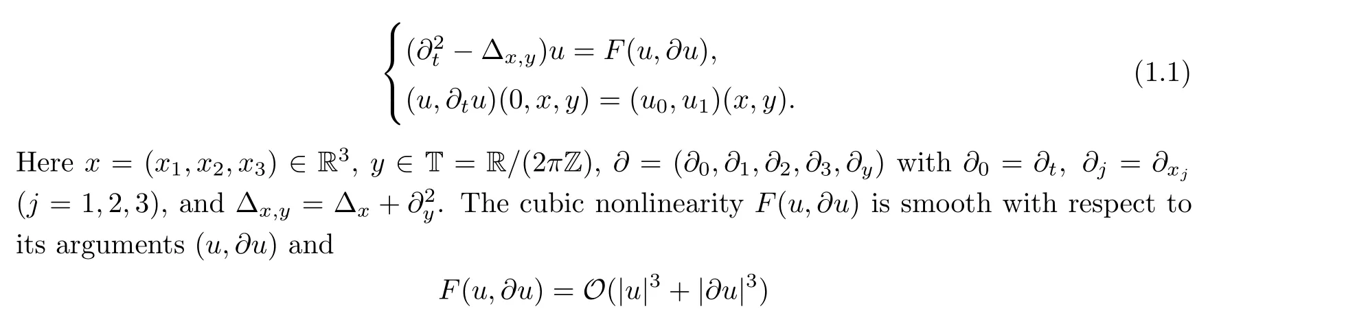
near (u,?u)=(0,0).
1.1 Notations and Main Result
To present the main result,we introduce some necessary notations for partial Fourier transformations, and the Sobolev spaceHm(R3×T), as well as various weighted functional spaces.
As in [31], the partial Fourier transformations off(x,y)∈L1(R3×T) are denoted by

In addition,we set the following conventions: fors ∈R,[s]is denoted as the largest integer that is not larger thans;Z*:=Z{0};the universal constantCin the estimates may vary from line to line.
Using the preparations above, our main result can be stated as follows:
Theorem 1.1ForN ≥13 and 0<θ <1/2, when the compactly supportedu0andu1satisfy that
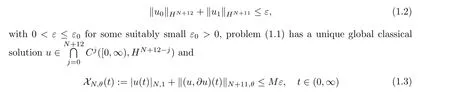
for some positive constantM.
1.2 Background and Some Related Results
We now review some results related to wave equations on product spaces.Consider the Cauchy problem of the quasilinear second order hyperbolic equation on R1+n×Tl(n ≥1,l ≥0):
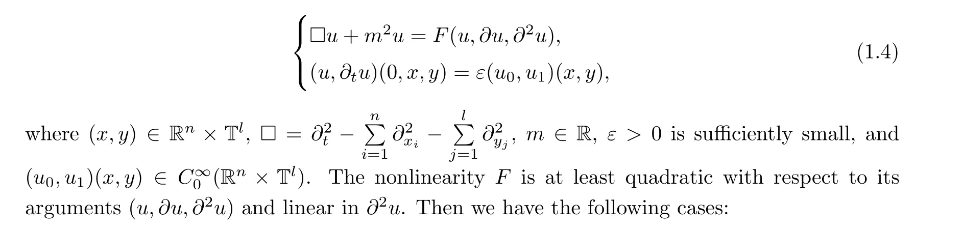
·m/=0,l=0.
In this case, the equation in (1.4) is the well-known Klein-Gordon equation; its global wellposedness for a smooth small-amplitude solution has been achieved for all spatial dimension.See[26,37]forn ≥5,[27,38]forn=3,4,and[36,40]forn=2.Whenn=1,the corresponding global well-posedness result relies on the null condition of the nonlinearityF(see [12, 42]).
·m/=0,l/=0.
To the best of our knowledge, there are few global well-posed results for this case.In[20, 21], the authors proved the global existence of a small data solution for the semilinear Klein-Gordon equation (?2t-Δx,y+1)u=±|u|p-1uwithp >1,n ≥1,l=1,2, andn+l ≥3.Recently, Tao and Yin established the global existence of a smooth small data solution for problem (1.4) in [41] forn= 3 andl= 1.Later, the authors in [31] obtained almost global smooth small-amplitude solution of problem (1.4) forn=2 andl=1.
The case for initial data posed on the purely periodic setting (i.e.,n= 0) is complicated,due to the lack of any dispersive property of the solution; see [6-8, 11, 13], etc..
·m=0,l=0.
In this situation, the equation in (1.4) becomes the wave equation.It is well-known that(1.4) has a global smooth small data solution forn ≥4; see for instance, [18] and [26].Meanwhile, forn= 3, the works of John [23, 24] show that the finite-time blowup for the smooth solution of (1.4) can happen with a certain quadratic nonlinearity.Klainerman [28] introduced the null condition on the quadratic nonlinearity and proved global well-posedness by the method of Klainerman’s vector fields; see also [9] for global existence result achieved by the conformal method.The cases forn= 1,2 are more intricate, we refer the reader to[3, 4, 10, 15, 22, 30, 33, 43, 44] and the references therein for the global well-posedness results.With respect to the finite-time blowup forn= 1,2, the reader can refer to Alinhac [1, 2] and Lai, Schiavone [34].
·m=0,l/=0.
In this case, only a few partial results are known regarding the long-time well-posedness of problem (1.4).Forn= 3 andl= 1, in [19], the authors obtained the global existence for a system of quasilinear wave equations with quadratic semilinear nonlinearities that are linear combinations of null forms.In the current paper, we study problem (1.1)on R1+3×T with the cubic nonlinearity.In [19], the authors employed the delicate hyperboloidal foliation method to prove the global existence.Compared with [19], the aim of our article is to directly use the conventional vector fields method, mainly by ingeniously combining the decay estimates due to Georgiev, with the weighted energy estimates.
1.3 Comments

The temporal decay estimates are motivated by Georgiev [16, 17], who showed that (1+t)u0;inh(t,x) and (1+t)3/2u±1can be controlled by the resulting nonlinearities through the weightedL2-L∞estimates.These two estimates play a key role in establishing our temporal decay estimate for the linear problem on the product space.When|n|≥2, we use the scaling skill to establish the decay estimate ofun(t/|n|,x/|n|); that satisfies a Klein-Gordon equation with unit mass.In this way,then-dependent decay estimate ofuncan be established explicitly.Based on the estimate of each Fourier modeun(n ∈Z), we consequently obtain the temporal decay estimate of the solutionu(t,x,y) of (1.1).On the other hand, the weighted energy estimate is closed in the framework of the product space with the help of the conformal energy inequality and the nonlinearity with a cubic form.Then a bootstrap estimate ofXN,θ(t)follows accordingly, and this leads to the global well-posedness.
1.4 Organization
In Section 2, we establish the pointwise decay estimate and the energy estimate for the linear problem by using two results of Georgiev and the scaling technique.In Section 3, we apply the linear estimates obtained in Section 2 to the nonlinear problem and complete the proof of Theorem 1.1.
2 Decay Estimate and Energy Estimate for the Linear Problem
In this section, we will establish the fundamental pointwise decay estimate and the energy estimate for the linear version of problem (1.1); this serves as the prototype for investigating the nonlinear version in the next section.More precisely, we consider the following Cauchy problem of the linear wave equation:
Here (t,x,y)∈R+×R3×T,g,handFare smooth functions with
for some positive constantR.
Using the notations in Subsection 1.1,we formally take the partial Fourier series expansions

2.1 Decay Estimate for the Linear Problem
In this subsection, we derive the pointwise decay estimate for the smooth solutionwof problem (2.1).
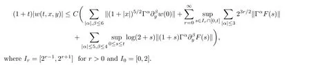
Proposition 2.1The smooth solutionwof problem (2.1) satisfies the estimate
The proof of Proposition 2.1 is based on the estimate of each Fourier modewn(t,x).As a first step, we deal withw0in (2.4), which exactly satisfies a wave equation.According to(2.4)0, we can decomposew0into two parts:

With the estimates obtained in the above two cases, we can finish the proof of Lemma 2.3.□
In view of Lemmas 2.2 and 2.3, we arrive at
Lemma 2.4The solutionw0of problem (2.4)0satisfies that
The estimates ofw±1below were also established by Georgiev.
Lemma 2.5(see [16, Theorem 1]) The solutionsw±1of problem (2.4)±1satisfy that

Based on the estimates shown in Lemmas 2.4 and 2.5, we can begin proving Proposition 2.1.


Finally, Proposition 2.1 follows from Lemma 2.4 and the estimate (2.12).□
2.2 Energy Estimate for the Linear Problem
In this subsection, we aim to establish the energy estimate for the smooth solution of problem (2.1).
First, we recall the classical conformal energy inequality.
Lemma 2.6(see [5, Theorem 6.11]) Withw0(t,x) as a solution to the linear inhomogeneous wave equation

ProofThe proof is divided into a series of estimates for the Fourier modes in (2.3).
i) Estimates of the zero-modew0(t,x).
By the standard energy estimate for the wave equation, we obtain from (2.4)0that

Here, the last inequality comes from the finite speed of propagation property ofw0(x,s) (since the initial data have compact supports, the finite speed of propagation property ofw0(x,s)implies that|x|≤s+Rfor some fixed constantR).Combining (2.14) with (2.15) yields that
ii) Estimates of the non-zero modeswn(t,x) (n ∈Z*).
Similarly, by the standard energy estimates for the Klein-Gordon equations, we get from(2.4)nthat

Finally, the estimate (2.13) comes from (2.18) and (2.19), and this finishes the proof of Lemma 2.7.□
3 Proof of the Main Result
In this section, we apply the linear decay estimate and the energy estimate established in Section 2 to analyze the nonlinear problem (1.1), and to build up our main result.
3.1 Decay Estimate and Weighted Energy Estimate for the Nonlinear Problem
We first establish thea prioridecay estimate for the solutionuof problem (1.1).
Lemma 3.1Under the assumptions in Theorem 1.1, the smooth solutionuof problem(1.1) satisfies that

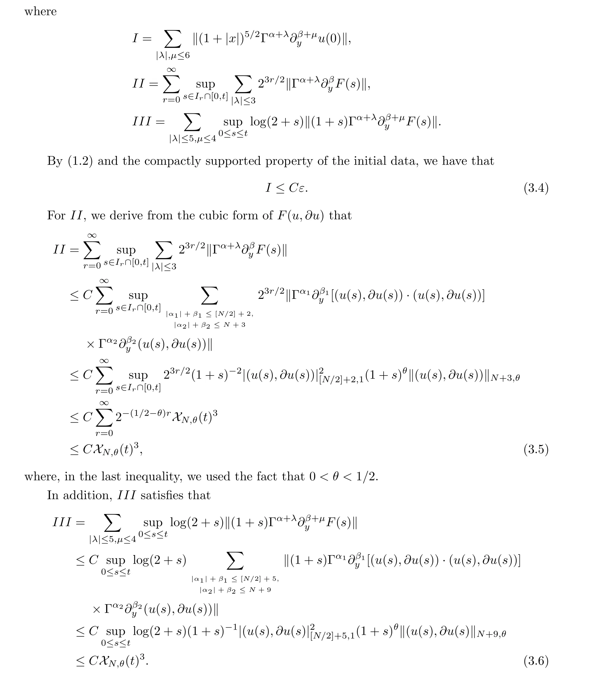
Finally, Lemma 3.1 is obtained by using of the estimates in (3.4)-(3.6).□
We next show thea prioriweighted energy estimate of the solutionuof (1.1).
Lemma 3.2Under the assumptions in Theorem 1.1, we have that
as long as the solutionuexists.
ProofUsing (1.1), (3.1) and Lemma 2.7, we see that

Then Lemma 3.2 follows from (3.7)-(3.9).□
3.2 Proof of Theorem 1.1
Proof of Theorem 1.1Now we finish the proof of Theorem 1.1 by a continuity argument.LetMbe a positive number to be determined later, and define that

AcknowledgementsThe author is deeply indebted to his advisor Professor Huicheng YIN for the guidance and encouragement.
Conflict of InterestThe author declares no conflict of interest.
 Acta Mathematica Scientia(English Series)2024年1期
- Acta Mathematica Scientia(English Series)的其它文章
- THE EXACT MEROMORPHIC SOLUTIONS OF SOME NONLINEAR DIFFERENTIAL EQUATIONS*
- SOME NEW IDENTITIES OF ROGERS-RAMANUJAN TYPE*
- NADARAYA-WATSON ESTIMATORS FOR REFLECTED STOCHASTIC PROCESSES*
- QUASIPERIODICITY OF TRANSCENDENTAL MEROMORPHIC FUNCTIONS*
- THE LOGARITHMIC SOBOLEV INEQUALITY FOR A SUBMANIFOLD IN MANIFOLDS WITH ASYMPTOTICALLY NONNEGATIVE SECTIONAL CURVATURE*
- GLOBAL SOLUTIONS TO 1D COMPRESSIBLE NAVIER-STOKES/ALLEN-CAHN SYSTEM WITH DENSITY-DEPENDENT VISCOSITY AND FREE-BOUNDARY*