
A Novel Trajectory Tracking Control of AGV Based on Udwadia-Kalaba Approach
2024-04-15 09:37RongrongYuHanZhaoShengchaoZhenKangHuangXianminChenHaoSunandKeShao
Rongrong Yu,,, Han Zhao, Shengchao Zhen,Kang Huang, Xianmin Chen, Hao Sun, and Ke Shao
Dear Editor,
This letter is about an automated guided vehicle (AGV) trajectory tracking control method based on Udwadia-Kalaba (U-K) approach.This method provides a novel, concise and explicit motion equation for constrained mechanical systems with holonomic and/or nonholonomic constraints as well as constraints that may be ideal or nonideal.In this letter, constraints are classified into structural and performance constraints.The structural constraints are established without considering the trajectory control, and the dynamic model is built based on them.Then the expected trajectories are taken as the performance constraints, and the constraint torque is solved by analyzing the U-K equation.It is shown by numerical simulations that the proposed method can solve the trajectory tracking control problem of AGV well.
Introduction: In recent years, AGV-A kind of mobile robot,which is a nonholonomic mechanical system and a typical model of uncertain complex system, gradually plays a more and more important role.Around the modeling and control problems of AGV,domestic and foreign scholars have done a lot of research work, such as PID control [1], robust control [2], adaptive control [3], sliding mode control [4], fuzzy control [5], neural network control [6] and other control methods [7].
The problem of solving equations of motion for nonholonomic mechanical systems has been energetically and continuously worked on by many scientists since constrained motion was initially described by Lagrange (1787) [8].For example, Gauss [9] introduced Gauss’s principle, Gibbs [10] and Appell [11] obtained Gibbs-Appell equations, Poincaré [12] generalized Lagrange’s equations,and Dirac [13] provided an algorithm to obtain the Lagrangian multipliers.However, they are all based on the D’Alembert principle, that is the virtual displacement principle.For constrained mechanical systems, Lagrangian multipliers can be used effectively for constrained calculation.However, the application of this method is not easy, as it is often very difficult to find Lagrangian multipliers to obtain the explicit equations of motion for systems, especially for systems with a large number of degrees of freedom and non-integrable constraints.The D’Alembert principle works well in many situations, but it is not applicable when the constraints are non-ideal [14].Thus, Udwadia and Kalaba obtained a novel, concise and explicit equation of motion for constrained mechanical systems that may not satisfy the D’Alembert principle.It can be applied to constrained mechanical systems with holonomic and/or nonholonomic constraints as well as constraints may be ideal or non-ideal, which is called U-K theory [15].It leads to a new and fundamental understanding of constrained mechanical system and a new view of Lagrangian mechanics.
Compared with the conventional methods in the trajectory tracking control of AGV, the proposed method has essential differences.In this letter, the dynamic model of the AGV with a driving and turning front wheel is first established based on the U-K theory.Second,constraints are classified in a new way, which include structural constraints and performance constraints.The structural constraints are set up regardless of trajectories, and the dynamic model is built based on the structural constraints.The AGV’s desired trajectory is set as performance constraints.Third, the constraint torque can be obtained based on the U-K approach to realize the trajectory tracking control of the AGV.It is shown by numerical simulations that, by the proposed method, the AGV’s movements has high accuracy.
Theoretical description: Using the marvelous U-K theory, the novel, concise and explicit equation of motion for constrained mechanical systems can be derived in three steps [14].

whereA(q,q˙,t) (may or may not be full rank) denotes anm×nconstraint matrix andb(q,q˙,t) denotes anm×1 column vector.
3) The additional generalized forces are imposed on the system to ensure that the desired trajectory is satisfied.Due to the existence of additional generalized forces, the actual explicit equation of motion of the constrained system can be described as
M(q,t)¨q=Q(q,˙q,t)+Qc(q,˙q,t) (2)
whereQc(q,q˙,t) denotes the additionaln×1 “constraint forces”, that are imposedontheunconstrainedsystem.Our aim is to determineQc(q,q˙,t)atanytimet, for theQisknown.
In Lagrangian mechanics,Qc(q,q˙,t) is governed by the usual D'Alembert Principle which indicates that constraint forces do zero work under virtual displacement and therefore is considered ideal constraints.However, constraints can also be non-ideal, while nonideal constraints generate non-ideal constraint forces, such as friction force, electro-magnetic force, etc.If there are both ideal and non-ideal constraints in the system,Qc(q,q˙,t) can be expressed as

wherethe matrixB=AM-1/2, the superscript “+” denotes the Moore-Penrose generalized inverse, andcis a suitablen-vector that is determined by the mechanical system.
From (2)-(5), the general “explicit” equation of motion (including both ideal and non-ideal constraints) is
If the work done by constraint forces under the virtual displacement is zero, then=0.Equation (6) reduces to obey the D’Alembert principle, which means the general “explicit” equation of motion is
Thus, at each instant of timet, the constrained system subject to an additional “constraint force”Qc(t) is given by
Trajectory tracking control of AGV: Suppose that the absolut e coordinate system XOY is fixed on the planar of the AGV with three wheels, consisting of one front wheel and two rear wheels.The front wheel can not only drive, but also turn.The model is shown in Fig.1.The front wheel is independently driven by two DC servo motors for driving and turning respectively.Two rear wheels only have the role of supporting and guiding.The wheels contact with the ground is characterized by pure rolling and no slipping.The variables and parameters of AGV are shown in Table 1.

Fig.1.AGV with a driving and turning front wheel.
According to Newton’s law, we can get
The dynamic equation of the driving motor of the front wheel is
wherekdenotes thetransmissionsystemsgearratio;kmdenotes electromagnetic torqueconstantof thedriving/turningmotor;Radenotes armature resistance of the driving/turning motor;Va1denotes input voltage of the driving motor;J1denotes rotational inertia of the driving/turning motor;J2denotes rotational inertia of the front wheel about the rolling axis;B1denotes viscous friction coefficient of the driving/turning motor shaft;B2denotes viscous friction coefficient of the front wheels axle; the torque of the driving motor is
The effects of non-ideal constraints are ignored.Then, the driving forceFis dependent onudandr, then (10) is simplified as
For this AGV model
Then, we can get

Table 1.Weighting/Optimal Gain/Minimum Cost
Differentiating (14) with respect totyields
From (9), (12) and (15), we can obtain the first structural constraint
The dynamic equation of the turning motor of the front wheel is
whereVa2denotes input voltage of the turning motor;Idenotes rotational inertia of the AGV’s front wheel about the steering axis;B3denotes viscous friction coefficient of the front turning axle; the torque of the turning motor is
Here, the effects of non-ideal constraints are ignored.Then, the turning angular acceleration φ¨=w˙2is dependent onIandut, upon using relation (18) in (17), (17) is simplified as (the second structural constraint)
From (13), the constraint is given byx˙sinθ-y˙cosθ=0.Differentiating it with respect tot(the third structural constraint)
Furthermore, orientation angle of the AGV and orientation angular velocity of the AGV has the relationship
By combining (21) with (14), we can get
Differentiating (22) with respect tot(the fourth structural constraint)
Thus, (16), (19), (20) and (23) can be put into the form of (2), with
Based on (2), the constraint torque can also be described as
where
Comparing (4) and (25), we can get
When the AGV needs to move along a desired trajectory, driving motor and turning motor should generate corresponding torques respectively which are denoted by τ1and τ2.x2+y2=1.That is
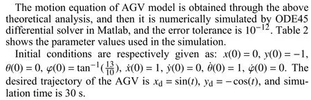
Numerical simulation: Suppose the AGV needs to track a circle:
Differentiating (27) twice with respect totto obtain the performance constraints of form (1) with
From (2) and (24), we know
where
Hence, the driving torque and the turning torque generated by the two motors respectively can be obtained by
The simulation results are shown in Fig.2, which shows that AGV can track a circular trajectory well by this method.
Conclusion: This letter proposes an AGV trajectory tracking control method based on U-K approach.In which, constraints are classified into structural constraints and performance constraints.The dynamic model is built based on the structural constraints, and expected trajectories are taken as the performance constraints.Through theoretical analysis and numerical simulation, it is proved that this method can solve the trajectory tracking control of AGV well.
Acknowledgments: This work was supported by the Shandong Provincial Postdoctoral Science Foundation (SDCX-ZG-202202029),the National Natural Science Foundation of China (52005302,52305118), and the Natural Science Foundation of Shandong Province (ZR2023QE003).
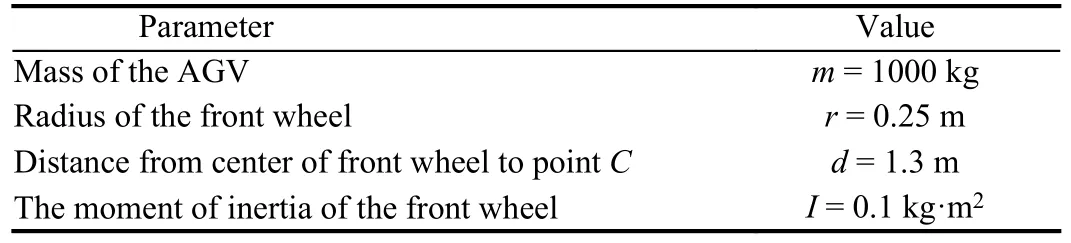
Table 2.The Symbol Definition of the AGV Variables and Parameters

Fig.2.The actual trajectory and the desired trajectory of the AGV.
 IEEE/CAA Journal of Automatica Sinica2024年4期
- IEEE/CAA Journal of Automatica Sinica的其它文章
- When Does Sora Show:The Beginning of TAO to Imaginative Intelligence and Scenarios Engineering
- Goal-Oriented Control Systems (GOCS):From HOW to WHAT
- Digital CEOs in Digital Enterprises: Automating,Augmenting, and Parallel in Metaverse/CPSS/TAOs
- A Tutorial on Federated Learning from Theory to Practice: Foundations, Software Frameworks,Exemplary Use Cases, and Selected Trends
- Cybersecurity Landscape on Remote State Estimation: A Comprehensive Review
- Data-Based Filters for Non-Gaussian Dynamic Systems With Unknown Output Noise Covariance