
SpinNet: Spinning convolutional network for lane boundary detection
2019-02-27 10:37RuochenFanXuanrunWangQibinHouHanchaoLiuandTaiJiangMu
Computational Visual Media 2019年4期
Ruochen Fan, Xuanrun Wang, Qibin Hou, Hanchao Liu, and Tai-Jiang Mu()
Abstract In this paper, we propose a simple but effective framework for lane boundary detection, called SpinNet. Considering that cars or pedestrians often occlude lane boundaries and that the local features of lane boundaries are not distinctive,therefore,analyzing and collecting global context information is crucial for lane boundary detection. To this end, we design a novel spinning convolution layer and a brand-new lane parameterization branch in our network to detect lane boundaries from a global perspective. To extract features in narrow strip-shaped fields, we adopt stripshaped convolutions with kernels which have 1×n or n×1 shape in the spinning convolution layer. To tackle the problem of that straight strip-shaped convolutions are only able to extract features in vertical or horizontal directions, we introduce the concept of feature map rotation to allow the convolutions to be applied in multiple directions so that more information can be collected concerning a whole lane boundary. Moreover,unlike most existing lane boundary detectors, which extract lane boundaries from segmentation masks, our lane boundary parameterization branch predicts a curve expression for the lane boundary for each pixel in the output feature map. And the network utilizes this information to predict the weights of the curve,to better form the final lane boundaries. Our framework is easy to implement and end-to-end trainable. Experiments show that our proposed SpinNet outperforms state-of-the-art methods.
Keywords object detection;lane boundary detection;autonomous driving; deep learning
1 Introduction
Object detection and segmentation are two of the most widely investigated areas of computer vision in recent decades. Generally speaking,advances in these domains are mostly driven by step changes made by classic baseline systems, such as Fast/Faster R-CNN[1, 2] and its follow-up architecture Mask R-CNN [3].These methods provide a general and conceptional platform which is both flexible and robust.
Autonomous driving is a concept that has the ability to define future transportation. Fully autonomous cars are currently a major topic for computer vision and robotics research, both academically and industrially.The goal of autonomous driving requires full control of the car, which in turn necessitates understanding the surroundings of the car by gathering information from sensors attached to it. One of the most challenging subtasks for such perception is lane boundary detection for car positioning. Lane boundaries differ from typical objects in having stronger structural features but fewer appearance clues [4]. For instance, lane boundaries often have long, continuous shapes, and are located at the bottom of the scene. Because of the lack of apperance clues, lane boundaries may be incorrectly detected if they mainly rely on local features. Additionally, occlusion is a significant difficulty for lane boundary detection, as in many scenarios, some parts of lane boundaries may be occluded by other objects, especially vehicles.
Given the above issues, it is essential to utilize global information for lane boundary detection so that lane boundaries can be predicted in a holistic way. One natural idea is to attempt to enlarge the receptive field of the network. Spatial CNN(SCNN) [4], inspired by RNN [5], proposed a sliceby-slice convolution method that is able to transfer information between neurons in the same layer. This architecture is also able to segment objects with long shapes. However, due to signal decay in the SCNN layer, distant information in the feature map is still hard to collect.
In order to gather and analyse features in large fields, in this paper, we present the idea of a spinning convolution and apply it within neural networks. The idea of a spinning convolution is to extract features along a narrow strip using a 1×norn×1 convolution layer. “Spinning” means that long kernel convolution can run at arbitrary angle. Because of the long kernel used in a strip convolution, features covered by the kernels can be equally collected without signal fading caused by long distances. Generally speaking,a straightforward strip convolution operation is performed only along a vertical or horizontal direction;however, the directions of lane boundaries or other slender detection targets can vary. As rotating strip convolution kernels to lie along arbitrary directions is difficult, we propose to instead rotate the feature maps to increase the number of ways of collecting features. In this way, a vertical strip convolution with a large kernel can process features along any direction.
Furthermore, most existing methods consider lane boundary detection as a segmentation problem,that is, predicting which pixels are covered by lane boundaries, and the final parameterized lane boundary curves are produced by a hand-crafted algorithm which takes the segmentation maps predicted by the neural network as inputs. But this sort of method may be confused when the lane boundary mask is irregular in shape. For instance, they have problems processing masks with “holes”. Instead, our approach carries out lane boundary detection by introducing a parameterization branch. To explicitly force the network to predict lane boundaries from a global perspective, our parameterization branch predicts the coefficients of lane boundary curves rather than segmentation masks. The final predicted lines are weighted combinations of the curves produced by the parameterization branch. To demonstrate the effectiveness of our proposed framework, we evaluate our results on the CULane dataset. We show that our SpinNet improves all prior lane boundary detection methods. To further verify the importance of our proposed spinning convolution and parameterisation branch, adequate ablation analysis is conducted. It reveals that both of the new operations contribute evidently to the overall performance.In summary, our proposed approach contains the following contributions:
·A spinning convolution operation which can extract long range features running in arbitrary directions, without information decay.
·A novel method of determining parametric lane boundaries using information from all the pixels in a feature map.
·An end-to-end lane boundary detection framework, called SpinNet, which achieves state-of-theart performance.
2 Related work
In this section, we briefly introduce some previous approaches closely related to our work.
2.1 Traditional methods
Traditional lane boundary detection algorithms are based on highly-specialised and hand-crafted low level features [6—10]. Methods exploiting structure tensors[11], color-based detectors [12], and bar filters [13]have achieved reasonable results; they are typically combined with Hough transforms [14] or Kalman filters [13]. When using such traditional techniques,post-processing is needed to weed out false detections,and to cluster lane boundary segments into final lines[7]. The weakness of traditional methods is that the models cannot handle complex circumstances. For example, occlusion, which is ever-present in real data[4, 15], presents difficulties for pattern-recognitionbased methods: filters extracting image features fail.Traditional methods are insufficient to process the complex situations required in real driving conditions.
2.2 Neural-network-based methods
Deep learning has recently become mainstream in this domain due to its better results [16, 17].The perception module in traditional approaches is replaced by a neural network, to overcome problems mentioned above. Huval et al. [18] proposed a deep learning based work, but lacked suitable large scale datasets for training. Spatial CNN [4] is now the state-of-the-art solution. It uses a specially designed architecture of convolution layers, enabling message passing between pixels across rows and columns in a layer. This paper also provided a brand-new large scale dataset. However, the limited number of message passing directions resulted in problematic lane boundaries with unsatisfactory directions.
Methods predicting lane boundaries with the assistance of other information are now a new trend.For instance,some research[19,20]has indicated that continuous driving scenes could provide information to constrain the predicted lane boundaries. However,these works place significant demands on dataset preparation. 3D vision has also been introduced to the lane boundary detection domain [21, 22] with reasonable results, but a major problem remains the costliness and rarity of both devices and datasets.Lee et al. [23] proposed a new way of predicting vanishing points to guide lane boundary prediction,giving a new approach to object-guided lane boundary segmentation.
2.3 Lane boundary parameterization
LaneNet [24] proposed a lane boundary detection framework that tackles the lane boundary detection task as an instance segmentation problem and also parametrizes the lane boundary by training an H-Net for view transformation. However, this work does not make good use of the predicted parameters,which are only used to generate the output,and are not capable of end-to-end training. Other works like Refs.[25,26]utilized similar methods, fitting a parabola or spline for each lane boundary, but some lane boundaries are so irregular that such curves cannot provide a good fit.
2.4 Feature map deformation
A common method [27] is to rotate the convolution kernel, making the output of the neural network rotationally invariant. However, features of long strip shape are needed to detect the lane boundary,rather than rotational invariance, in our approach.Rotational invariance is typically of benefit in limited specific situations, like fingerprint recognition [28],galaxy morphology prediction [29], etc. When using the message passing technique of Spatial CNN[4], we have to find another solution.
3 SpinNet
In this section, we propose a framework for lane boundary detection and positioning, called SpinNet.SpinNet introduces two new ideas that are easy to implement.
3.1 Overall structure
SpinNet is an end-to-end trainable neural network,which employs VGGNet [30] as its backbone model.The structure is shown in Fig. 1. To ensure high resolution in the output feature map, we discard all fully-connected layers and the last two pooling layers (pool4 and pool5) and change the dilation rates of all convolution layers in stage 5 from 1 to 2 to enlarge the receptive field. The proposed spinning convolution layer,whose purpose is to extract features along a long narrow field in a series of directions, is deployed after conv5 in VGGNet. After the spinning convolution layer, we also use a Spatial CNN layer,following Ref.[4],to further enlarge the receptive field.A fully-connected layer, followed by a softmax layer,is then used to predict a lane boundary presence vectorei, representing the probability that theith lane boundary is present in the image. After upsampling the feature map to the same size as the input image, a convolution layer predicts a map giving the probability of pixels being covered by lane boundaries, a coefficient matrix determining the parameters for the curves belonging to each pixel,and a coefficient confidence map.
3.2 Spinning convolution layer
Classical convolution kernels are usually square, e.g.,3×3,5×5,etc. Using larger square kernels can enlarge the receptive field of a network. However, using huge square convolution kernels would lead to unacceptable computational costs in our specific task if we wish to cover a lane boundary. Furthermore, square convolution layers would have so many parameters in the convolution kernel,making them difficult to train.In practice, a lane boundary only occupies a small proportion of a square area, as they are narrow strips.A better approach to detecting these objects is to use strip-shaped narrow convolution kernels, e.g., 1×norn×1.
To collect information about objects, Spatial CNN[4] borrowed ideas from RNN, passing messages inside its layers. However, its critical weakness is the message decay occurring in its message passing procedure.
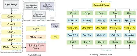
Fig. 1 The network structure of SpinNet and an illustration of the proposed spinning convolution. (A) shows the whole network structure of SpinNet, in which Conv_1 to Dilated_Conv_5 are VGGNet backbone and the elements in dotted box and “Existence Vector” are the output of SpinNet.
Our specially-designed convolution kernels possess three clear advantages compared to square-shaped convolution kernels and the SCNN technique. First,strip-shaped kernels provide a set of long narrow receptive fields in a series of directions. Second, these kernels require fewer network parameters: while a convolution layers with 3×3 and 9×1 kernels have the same number of network parameters, the latter has a much bigger receptive field than the former for the specific task of lane boundary detection. Third,our kernels are decay-free so that no information will be easily lost.
But lane boundaries are not just in these two specific directions, namely horizontal and vertical—they are arbitrary in direction. To overcome this problem, we have designed a method of rotating feature maps: the tilted lane boundaries become vertical or horizontal in one of the rotated feature maps, allowing them to be detected by vertical or horizontal convolution kernels. Although lane boundaries may not always be straight, some certain long strip kernels possessing different angles in variant positions of the feature map can fit a curve properly.Combining the above two concepts in a single layer gives our spinning convolution layer. Sample outputs of our spinning convolution are shown in Fig. 2.
The architecture of this spinning convolution layer is based on an original convolution layer, in which we replace the square convolution kernels by our specially designed strip kernels,and initially,we get the feature map generated by the backbone network. We first pad the feature map, and the rotation operation is then applied to the padded feature map, using a series of angles. Each different angle gives a new padded and rotated feature map. The strip convolution layer is then connected to each of these feature maps, which generates a series of new feature maps. We then perform an inverse rotation operation on each, and crop out the padding. Finally, we concatenate these outputs to form the final output of our spinning convolution layer. The process described above is shown in Fig. 1(B), in whichαis a super parameter determining the spinning angle. We use five spinning convolutions with differentαto form a spinning convolution stack.
Before our approach, there are many traditional approaches that aim to collect straight lane boundary information. However, there are several lane boundaries in one input image, and the boundaries may have some spatial information, or even correlations with each other. Thus, cropping the input to detect a lane boundary object is improper,for it will omit spatial information and correlations.Additionally, if we perform featuremap/input-picture rotation at the beginning of the network, we will not be able to finish the strip-shaped convolution, thus not be able to collect information on various directions explicitly. As we mentioned above, the directions of our strip-shaped kernels are fixed into 2, namely,horizontal and vertical. Thus, rotating feature maps is the very method to perform convolution using stripshaped non-horizontal/vertical kernels, and this is our original purpose to perform this rotation.

Fig. 2 The result feature maps of spinning convolution. Given the strip-shaped kernels, performing convolution in traditional way can only use horizontal and vertical kernels. But in our purposed method, kernels can be designed to spin at arbitrary angles, as shown in the upper-right corner of each feature map. (a) is the original image input. (b–f) are the output feature maps of the spinning convolution stack. Each of the feature maps has 64 channels and the mean values of them are shown. The kernels are rotated with -60, -30, 0, 30, 60 degrees respectively.Obviously, a kernel with a certain rotation angle can collect more edge information of lane boundaries in that direction.
It seems that our method, rotating the feature maps,will receive a better result compared with these traditional techniques, since the spatial information and the correlation between lane boundaries are properly preserved, while the increase in calculation just arises a little.
3.3 Parameterization branch
Various works [24—26] consider lane boundary parameterization as a problem of fitting the lane boundary with a spline or parabola. However, all of the above methods share two common defects.Firstly, lane boundary parameterization is treated as a separate process from lane boundary semantic segmentation. In fact, the existing parameterization process is a hand-crafted algorithm only using the segmentation mask as input—it is unable to exploit the rich information in network feature maps. Instead,the spatial information from these two tasks can be exploited simultaneously inside the network, so that the tasks of lane boundary prediction and coefficient prediction can work together to provide mutual assistance, and the network will be an end-to-end task in this way. In our method, we combine these two tasks into one end-to-end network. Secondly, all previous works predict only a single set of coefficients,i.e., a single curve, for a lane boundary in an image.Commonly, lane boundaries are long smooth shapes,but in complex situations, their trajectories may be highly curved or irregular. Fitting a single curve with simple few global coefficients, typically a low order curve,will not give satisfactory results. In these situations, it is necessary to predict lane boundary curves locally, and then concatenate these local curves into the final complex lane boundary. We demonstrate later how we solve this problem.
We mitigate the first defect by combining parameterization and segmentation into one organic system: we generate two results using two branches attached to the same backbone. During training,gradient back-propagation influences the backbone through two paths: a semantic segmentation branch and a parameterization branch, allowing it to utilize the rich information included in the feature map for both tasks.
To alleviate the second defect,we force the network to predict not only local probability information, but global curve coefficients in each pixel of the feature map. By doing so, we explicitly make every pixel predict the curve from a global perspective.
After computing curve coefficients pixelwisely,the next step is to acquire global lane boundary information from this information. First, we know curve could be represented by a set of coefficients.Let these coefficients beP0,··· ,Pn. The curve
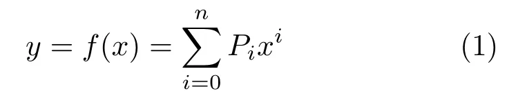
then represents that lane boundary.
Let us first define the local curve. Unlike the global curve whose origin is at the upper left of the image,the origin of the local (relative to a certain pixel)curve is at the corresponding pixel in the image itself.

Fig. 3 The curve aggregation pipeline. (a) shows a part of an input picture. There are 4×4 grids, and each grid indicates one pixel in the output feature maps and a square area in the original picture. The green horizontal line is the virtual baseline we are trying to solve the intersection point on. A grid is in orange only if the grid has the maximum Mi on a horizontal vertical baseline. (b) shows the separate curves Qi generated from the four orange grids. These curves have intersections xi,2 with the green horizontal baseline, which are shown in (c). These intersections are summed after being weighted by their confidence M and the distance between their baselines and the green one, generating the final answer x2 on the green baseline. Repeat this process, we get all the xjs, and then we perform a simple post-process to draw the predicted lane boundary in orange shown in (d).
Overall, we first treat the whole lane boundary as a combination of several local curves, which is simple to generate from the dataset by polynomial fitting.As the dataset provides some key points on the lane boundary, we choose one key point and its neighbors,to determine the local curve coefficients near that key point by polynomial fitting. As for other key points,the method is similar. This is a simple pre-processing task by which we generate the ground truth of the lane boundaries coefficients. Then, we add a branch in parallel with the existing segmentation branch. Its aim is to generate the local curve coefficients at each pixel.
The method used to generate the set of coefficients of a lane boundary is regular,and could be performed by simply adding several dense layers after the output.But this method will let spatial information from the feature map be lost. Instead, for each pixel,the coefficients of the local lane boundary are easy to predict as this prediction only require adjacent information. Furthermore, the accuracy of local prediction is much better since one pixel only needs to predict the lane boundary nearby. We can thus use a feature-map-based pixelwise coefficient computation branch.
As the network only predicts local coefficients and the global coefficients are easy to acquire from the dataset,we need a simple global—local transformation.And this can be performed by

wherefkis the local curve function whose origin is at pixelk:(xk,yk). Solving the equation above,we can easily get the new lane boundary curve coefficientsPk,i, with origin at pixelk. Preliminary experiments showed that usingn= 1, i.e., fitting straight lines to lane boundaries, is not sufficient, but on the other hand, usingn >2 makes imperceptible further improvement. Thus we setn= 2, i.e., fit parabolas. In our approach, a parameterization branch is connected after the output layer of our backbone to produce a pixelwise coefficient matrix.
Some may believe there is a paradox that our output has passed the spinning pipeline, and thus only straight edge information was preserved, which is a misunderstanding. The shape of the convolution kernels only indicates the shape of the sampling points, and the ability to predict objects in other shapes will not be lost. In Section 4, we proved by experiments that strip-shaped convolution kernels have a better capability of detecting lane boundaries.
3.4 Curve aggregation
In the above introduction, we could get the local coefficient matrices generated by the neural network.That is, for each pixel of the feature map, there are a set of coefficients indicating the local lane boundary curve. To merge the set of local curves into final lane boundaries, we design the curve aggregation algorithm.
Curve aggregation is a weighted averaging process.For a point (x,yi) which lies in the virtual horizontal baseliney=yiin the final lane boundary, the target coordinatexis the weighted average of the horizontal ordinates of the intersections of the local curves and the virtual baselines. The weights are positively correlated with the confidence of local curves predicted by the network and are negatively correlated with the distance between the pixel and the virtual baselines. Therefore, the more accurate the curve is, the more contribution the curve makes to the final lane boundary. Besides, every pixel is mainly responsible for the section of the final lane boundary close to the pixel. Therefore, we proposed the following method to generate the key points of a lane boundary.
So far,the parameterization branch has provided:a probability mapwhereMiis the probability that pixeliis covered by the final lane boundary andNCis the number of pixels,a coefficient mapP ∈RNC×3wherePiis the vector of coefficients of the curve ati, and a confidence mapF ∈RNC,whereFiis the confidence in the curve coefficients atias predicted by the network. Detailed defination and implementation of confidence mapFicould be found in Section 3.5. We process the four lane boundaries separately,so from now on,we splitinto four slices,process each sliceM ∈RNCseparately. As we can exploitto achieve the availability of reusingFandPin different lane boundaries, so it is unnecessary forForPto possess four channels.
We first setNbvirtual horizontal baselines evenly located in the image, aty=j×C, j=0,...,Nb-1 whereCis the baseline interval. The result of our algorithm is several points lying on the virtual horizontal baselines. For each baseline, we find the maximumMi. The corresponding values ofiindicate the pixels most likely to be in the lane boundary,so we call them key-points from now on. However,we ignore any such points for whichMiis below a threshold,as they are unlikely to be covered by a lane boundary. LetKias thei-th key-point, withyvalueyKi. For each key-pointKi, we can get the curveQKiassembled byPKi. These curves in general have several intersections with at least some of the virtual horizontal baselines. Let thex-coordinate of the intersection ofQKiandy=j×C, j=0,1,...,Nb-1 bexKi,j. The coordinatexjof the result fory=j×Cis given by

whereαis a constant. Thus, (xj,jC) is one of our result points. After finding such points for all virtual horizontal baselines, the set of (xj,jC) is then the final output.
3.5 Loss function
The loss functionLshould have the ability to refine the probability maps and the coefficient maps simultaneously. To do so, it must be a weighted sum of multiple parts:

where the weighting coefficients are hyperparameters which must be tuned.
The first part of the loss is the lane boundary object binary segmentation lossLossbin. To compute it, we can easily calculate a softmax cross-entropy between prediction and the ground truth in the semantic segmentation task. The second part of the loss is the lane boundary existence lossLossex. This essentially concerns a binary classification task, so again a crossentropy computation suffices. The third part of the loss is the lane boundary coefficients lossLosspar. In one step of forward propagation, after finding ˉM, we are able to categorize each pixel. Thus, if a pixelkbelongs tolane boundary j, its coefficientsPishould be as close to the ground truthPi,gt,j,kas possible.Here,Pi,gt,j,kstands for the ground truth coefficientsPifor lanej, transformed to origin atk. We may then calculate the loss as follows:

where|·|denotes theL1loss. As we treat the curves as parabolas, in the following we simply replaceP2bya,P1byb, andP0byc.
There are two tasks at each pixel to perform,to predict the semantic segmentation of the lane boundary, and to predict the confidence in the coefficients of the lane boundary passing through it. While it seems obvious that these two tasks are connected, they do not in fact constitute a sound causal relationship, as pixels with precise coefficients prediction may lie outside any lane boundary. So, we need a measurement of the confidence of coefficients accuracy as the contribution factor mentioned in the previous section. At pixelk, the ground truth valueFgt,j,kfor lane boundaryjand origin at pixelkis defined as follows:

Our experiments indicate thatbandcare essential to lane boundary prediction, and the loss forbandcis key to determining the confidence.
The loss function forFis easy to compute:

We can then get the total loss:
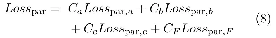
whereCs are the hyperparameters to finetune.
4 Experiments
In this section,we show the efficacy of SpinNet on the large-scale CULane dataset. Comparisons with stateof-the-art methods show that our proposed framework outperforms all prior lane detection methods. To further analyze the effectiveness of each component of SpinNet, we have performed a series of ablation experiments, and the effects of some key hyperparameters also are shown.
4.1 Implementation details
4.1.1 Training and testing
Images provided by datasets only have points located evenly on each of the lane boundaries. To generate ground truths for lane boundary coefficients, we performed parabola fitting to these point sets.
During training, the original image, binary masks of corresponding lane boundaries, lane boundary existence vectors, and curve coefficients sets are fed into our end-to-end network. During testing, in order to judge if a lane boundary is correctly detected,we regard the lane boundaries as polyline segments with a width of 30 pixels, and then calculate the intersection-over-union (IoU) between the ground truth and the prediction. Predictions whose IoUs are greater than a certain threshold (0.5) are regarded as true positives (TP). This enables us to assess our method using the F1 measure.
4.1.2 Hyper-parameters
Our proposed network was implemented on TensorFlow [31]. The input images were not augmented. The hyper-parameters are set as follows:momentum (0.9), learning rate (0.05), weight decay(0.0001). We trained our network on a single Nvidia GTX1080 Ti GPU for 180k iterations.
4.2 Ablation study and setup
4.2.1 The effect of spinning convolution and parameterization branch
To evaluate the effectiveness of spinning convolution,we replaced this operation by a traditional convolution stack. The results in line “w/o Spin-Conv” of Table 1 indicate that spinning convolution contributes 1.1 percentage points to the overall performance.
To evaluate the effectiveness of our lane boundary parameterization branch, we disabled local curve prediction in our model and extracted curves from lane boundary segmentation masks,following existing methods such as SCNN [4]. The results in line“w/o Parameterization” of Table 1 indicate that the parameterization branch benefits evidently to lane boundary detection performance.
We also disabled both operations; the inferior experimental results further demonstrate the effectiveness of our proposed operations.
4.2.2 Spinning angles
To better understand our spinning convolution layer and suggest the best way to use it, we determined how choice of spinning angles affected the results. We used 3, 5, 7 simultaneous spinning convolutions in each experiment, with angles chosen as in Table 2.The experiment indicates that rotation angles affect lane boundary detection performance. Only a small spinning angle cannot give us the best result.Moreover,too many or too few directions of rotations will also harm the performance. The experiments show that (±60°,±30°,0°) is the optimal angle settings we have found, implying that making the spinning angles evenly distributed is a good strategy.
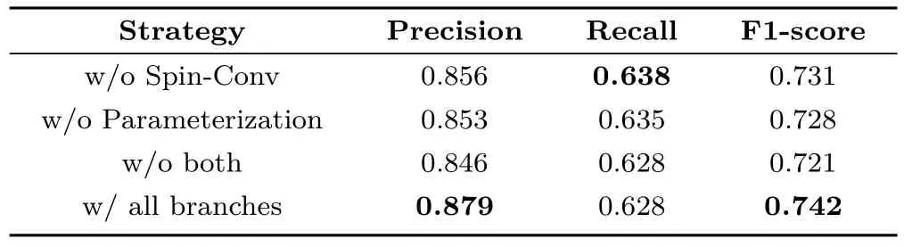
Table 1 Ablation study of our proposed SpinNet. “w/o Spin-Conv”represents the performance when spinning convolution is replaced with traditional convolution stack. “w/o Parameterization”means disabling parameterization branch and generates lane boundary prediction results from segmentation mask. The experiments show that SpinNet achieves best performance when both proposed branches are used

Table 2 Performance of SpinNet when using different rotation angles in spinning convolution. (±20°,±10°,0°) means that there are five sub-branches in spinning convolution stack, with rotation angles from-20° to 20°
4.2.3 Spinning convolution kernel size
A kernel of size 1× nis used in the spinning convolution, and its sizencontrols the range of the receptive field of this convolution layer. In theory, a large receptive field usually benefits performance,but requires more parameters which may increase training difficulty. We performed an experiment to find the optimal size of spinning convolution kernel. The results are shown in Table 3. The results reveal that a kernel of size 12×1 achieves the best result. A shorter or longer kernel harms the overall performance.

Table 3 Performance of SpinNet when using different size of stripshaped large kernel in spinning convolution. The size of the kernel we use is 1×n. The experiment reveals that too long or too short kernels harm the performance, and a 1×12 kernel is most appropriate for our task
4.3 Comparison with state-of-the-art
We compared our proposed method with existing lane boundary detection methods using the CULane dataset. Table 4 lists the results; performance is measured by F1-score. This table also gives efficacy comparison in some particular scenario. It is clear that our new approach, SpinNet, achieves the best overall results, improving on the baseline result presented in Zhang et al. [34] or LineNet [35] by 1.1 percentage.
In addition to quantitative evaluation, some visualization results are shown in Fig. 4. We label ground truth lines in green, true positive predictions in blue,and incorrect predictions in red. Our SpinNet is able to handle crowded road with evident occlusion.For failure cases, we find that it is difficult to detect lane boundaries fully occluded by cars.
5 Conclusions
This paper has presented a lane boundary detection framework, including a novel spinning convolutionlayer and a new lane boundary parameterization branch. The spinning convolution layer with strip kernel is able to extract features in long narrow fields along a series of directions. The parameterization branch predicts a whole curve for each pixel in the output feature map. Experiments show that both operations improve the performance of a lane detection network, and that the proposed framework outperforms prior methods on the CULane dataset.

Table 4 Lane boundary results on CULane dataset (F1-measure). The columns from “Normal” to “Curve” show the effectiveness comparison in some particular scenario. The column “Total” shows the overall performance in the whole test set of CULane dataset, indicating that our SpinNet achieves new state-of-the-art result

Fig. 4 Selected examples produced by our SpinNet. Green lines are the ground truths. Blue lines are the predicted true positive line boundaries, while red lines are the incorrect prediction results. From this figure, we can see that our framework works well even in crowded road with obvious occlusion and scenes with low contrast.
Acknowledgements
This work was supported by the National Natural Science Foundation of China (Project No. 61572264),Research Grant of Beijing Higher Institution Engineering Research Center, and Tsinghua—Tencent Joint Laboratory for Internet Innovation Technology.
Open AccessThis article is licensed under a Creative Commons Attribution 4.0 International License, which permits use, sharing, adaptation, distribution and reproduction in any medium or format,as long as you give appropriate credit to the original author(s)and the source, provide a link to the Creative Commons licence, and indicate if changes were made.
The images or other third party material in this article are included in the article’s Creative Commons licence, unless indicated otherwise in a credit line to the material. If material is not included in the article’s Creative Commons licence and your intended use is not permitted by statutory regulation or exceeds the permitted use,you will need to obtain permission directly from the copyright holder.
To view a copy of this licence, visit http://creativecommons.org/licenses/by/4.0/.
Other papers from this open access journal are available free of charge from http://www.springer.com/journal/41095.To submit a manuscript, please go to https://www.editorialmanager.com/cvmj.
 Computational Visual Media2019年4期
- Computational Visual Media的其它文章
- Practical BRDF reconstruction using reliable geometric regions from multi-view stereo
- Reconstructing piecewise planar scenes with multi-view regularization
- Evaluation of modified adaptive k-means segmentation algorithm
- Mixed reality based respiratory liver tumor puncture navigation
- InSocialNet: Interactive visual analytics for role–event videos
- Adaptive deep residual network for single image super-resolution