Calibration,validation,and evaluation of the Water Erosion Prediction Project (WEPP) model for hillslopes with natural runoff plot data

Shuyun Wng , Ryn P.McGehee , Tin Guo , Dennis C.Flngn b,,*,Bernrd A.Engel

a Department of Agricultural & Biological Engineering, Purdue University, West Lafayette, IN, 47907, USA

b USDA-Agricultural Research Service, National Soil Erosion Research Laboratory, West Lafayette, IN, 47907, USA

Keywords:WEPP Runoff Soil loss Calibration Validation

A B S T R A C T The Water Erosion Prediction Project(WEPP)model has been widely used for estimating runoff and soil loss.The evaluation of the latest version (version 2021.133) under a range of environmental conditions can provide confidence to its users.The objectives of this study were to evaluate the WEPP model for runoff and soil loss predictions using 1159 plot years of rainfall-runoff events data from field experimental plots with various climates, soils, topographies, and crops.WEPP runoff and soil loss predictions were compared to the observations before and after input parameter calibration.The results showed good predictions of runoff and soil loss were obtained with both the uncalibrated and calibrated WEPP model for all considered scales with Nash-Sutcliffe model efficiencies (NSE) over 0.4.The calibration of input baseline effective hydraulic conductivity (ke), baseline critical shear stress (τc), baseline rill erodibility (kr), and baseline interrill erodibility (ki) improved WEPP model performance with NSE values of 0.98 and 0.91 for average annual runoff and soil loss predictions,respectively.The WEPP model tended to underestimate the runoff and soil loss for large events with runoff over 100 mm and soil loss over 120 t/ha.Good event runoff and soil loss predictions(NSE ≥0.4)were obtained for the most common cropping/management systems considered, including corn, cotton, tilled fallow, and wheat after calibration.This study illustrates the most recent WEPP model's performance for runoff and soil loss predictions, and provides a comprehensive set of results.

1.Introduction

Soil erosion in agricultural systems is a worldwide issue causing the loss of fertile topsoil,sedimentation and the pollution of off-site surface water bodies.The prediction and quantification of soil erosion through computer simulation models have utility in evaluating land-use management and environmental planning and assessment (Tiwari et al., 2000).Numerous models have been developed to simulate the soil erosion process with a variety of parameters considered.Traditionally, the Universal Soil Loss Equation (USLE; Wischmeier & Smith, 1978) and the revised version of it (RUSLE; Renard et al., 1991) have been applied to predict the long-term average annual soil loss produced by rainfall erosion in many parts of the world(Kinnell,2017).Given the need to predict soil erosion over shorter time scales, physically-based models have been more recently developed to estimate soil loss from individual rainfall events by simulating the components of the erosion process.These models can potentially achieve a wider range of applicability in various environments such as agricultural lands, rangelands, forests, and urbanized areas (Mahmoodabadi &Cerdˋa, 2013).

The Water Erosion Prediction Project (WEPP) model (Flanagan et al., 2001) is a physically-based erosion computer simulation program,which has been used worldwide(Gr?nsten&Lundekvam,2006;Pandey et al.,2009,2021;Srivastava et al.,2020;Zheng et al.,2020).Many physical processes in soil erosion are included in the WEPP model including infiltration, runoff, raindrop and flow detachment, sediment transport, deposition, plant growth, and residue decomposition (Flanagan et al., 2007).This model can assess both the spatial variability and temporal variability of the soil erosion process.WEPP has been applied at both hillslope (Alewell et al., 2019; Gr?nsten & Lundekvam, 2006; Pieri et al., 2007; Yu &Rosewell, 2001; Zheng et al., 2020) and watershed (Dobre et al.,2022; Pandey et al., 2009; Shen et al., 2009; Srivastava et al.,2020) scales to estimate daily, weekly, monthly, annual or average annual values of runoff and soil erosion.Given the wide range of applications by the WEPP model, there is a continuing need to evaluate the performance of the latest version (WEPP version 2021.133) to determine model prediction efficiency.Soil erosion model evaluations are crucial for obtaining valid information on soil erosion processes and land management choices(Tekwa et al.,2021).

Given individual soil erosion processes are simulated in physically-based models,these models often can perform well with sufficient inputs even without calibration.The study of Tiwari et al.(2000) obtained acceptable runoff and soil loss results from uncalibrated WEPP simulations at similar levels to both USLE and RUSLE using a portion of the USLE datasets.However,Bhuyan et al.(2002) recommended calibration, which allows for the most accurate predictions with soil erosion models.Similarly, Yu et al.(2000) suggested that use of WEPP outside its U.S.database required calibration with locally obtained data.Through calibration of WEPP effective hydraulic conductivity, rill erodibility, and soil critical shear stress, Zheng et al.(2020) was able to satisfactorily predict soil loss on hillslopes with steep slope gradients in China.Pieri et al.(2007) also suggested calibration of the erodibility parameters in order to improve erosion predictions,as they reported underestimated results with the uncalibrated WEPP model.

When calibrating WEPP, the most often recommended input parameters to consider are effective hydraulic conductivity, rill erodibility, interrill erodibility and critical shear stress (Flanagan et al., 2012), though these are not the only parameters to which WEPP is sensitive.WEPP uses the Green-Ampt Mein-Larson equation modified for unsteady rainfall to calculate infiltration and runoff (Stone et al., 1995).The sensitivity analysis of the Green-Ampt equation parameters by Skaggs and Khaleel (1982) showed that the infiltration and runoff amounts were most sensitive to porosity and hydraulic conductivity.Moreover, a considerable improvement of WEPP runoff predictions was obtained by calibrating the effective hydraulic conductivity in Risse et al.(1994).In the study of Brunner et al.(2004),the sensitivity measurements of different soil input parameters indicated that the WEPP model was highly sensitive to changes in soil texture,which was caused by the model's calculation of soil hydraulic properties.The soil texture,organic matter,and rock content are used in pedotransfer functions to obtain soil hydraulic properties (hydraulic conductivity, rill erodibility, interrill erodibility, bulk density, field capacity, and wilting point).Pandey et al.(2008)showed that the sediment yield was highly sensitive to interrill erodibility and effective hydraulic conductivity.Nearing et al.(1990) concluded that WEPP runoff predictions were very sensitive to effective hydraulic conductivity and erosion predictions were sensitive to rill erodibility and critical shear stress.When considering the increased number of saturation-excess runoff events under conservation tillage and notill,the modified model WEPP-UI highlighted the importance of soil depth or the depth to restrictive layer,which helps to determine the infiltration-excess and saturation-excess runoff events (Boll et al.,2015).Rittenburg et al.(2015) categorized three hydrologic land types based on the soil depth and the depth to a restrictive layer.Their study observed different responses of these hydrologic land types to rainfall events, which also provided a framework for the application of the best management practice (BMP) for each hydrologic land type.Therefore, the calibration of soil depth and the depth to a restrictive layer can improve the WEPP model performance, especially when saturation-excess runoff events widely exist.An overall assessment of a soil erosion model needs to contain a range of diverse climatic, topographic, soil, and management conditions.Comparisons between performance before and after model calibration can evaluate how much WEPP predictions could be improved.The goal of this study was to evaluate the WEPP model performance in simulating runoff and soil erosion from natural rainfall/runoff field experimental plots.Specific objectives were (1) to compare WEPP predictions to observations from hillslopes before and after model calibration,and(2)to assess WEPP performance for different cropping/management systems.

2.Materials and methods

2.1.Data sets

A portion of the USLE database was used in this study.The USLE database contains data on runoff and soil loss for a large number of plots in the USA since the 1930s(Kinnell,2017).The history of this database is given at https://www.ars.usda.gov/midwest-area/westlafayette-in/national-soil-erosion-research/docs/usle-database/usle-history.Only natural rainfall events on natural runoff plots were recorded in this dataset.In this study, twenty locations from the USLE database with detailed climate, soil, topographic, and management information were considered for analysis, which are shown in Fig.1.The number of plots, slope gradients, soil types,crops,and recorded years for each plot are shown in Table 1.In total,there were 134 plots and 1159 plot years of data utilized for WEPP evaluation.Climate files contained the precipitation amount,duration,start time,and peak 5-min rainfall intensity for all events.Breakpoint rainfall data, a type of precipitation data in which precipitation characteristics are preserved to the degree of a given gauge's precision, were available for the events causing surface runoff.Soil files included the soil type and the soil texture with corresponding soil depth for each layer.All plots considered in this study were represented with a single overland flow element of a uniform slope gradient and width.Slope files contained the unique slope gradient, length, and width for each plot.For each plot, the type of crops, the date and type of tillage operation, and the crop yield were recorded.The USLE database included many of the most common crops in the United States including corn, soybeans,wheat,oats,cotton,and bromegrass.Various soil types and a wide range of slope gradients were considered in this data.For each plot,the runoff depth and soil loss amount were recorded for the events driven by natural rainfall.This study focused on the rainfall-driven events only and therefore, excluded any snowmelt-driven events.

2.2.WEPP inputs

The WEPP hillslope model requires four input files: climate,topography, soil, and management.The raw data from records at the USDA-ARS National Soil Erosion Research Laboratory (NSERL)were translated into WEPP input file formats by several researchers over many years.The WEPP model accepts either breakpoint format data or daily ‘ip-tp’ format data (intensity-at-peak factor and time-to-peak factor)climate input files(McGehee et al.,2020).In our study,the‘daily ip-tp format’was used given that breakpoint data were not available for all precipitation events.The WEPP modeling system includes a stochastic climate generator(CLIGEN)(Nicks et al.,1995),which produces daily estimates of precipitation,time to peak, peak intensity, storm duration, maximum and minimum temperature, dew point temperature, wind speed and direction,and solar radiation for a single geographic point(Srivastava et al.,2019).CLIGEN daily predictions are generated based on longterm observed weather station data statistics.In this study, given the lack of daily maximum and minimum temperatures,dew point temperature, wind speed and direction, and solar radiation, these values were simulated with CLIGEN.The CLIGEN-generated climate data was validated by previous studies and most of these plots were also used in Tiwari et al.(2000).The precipitation amount,time to peak, peak intensity, and storm duration values were those observed or calculated based on the climate records in the USLE database.

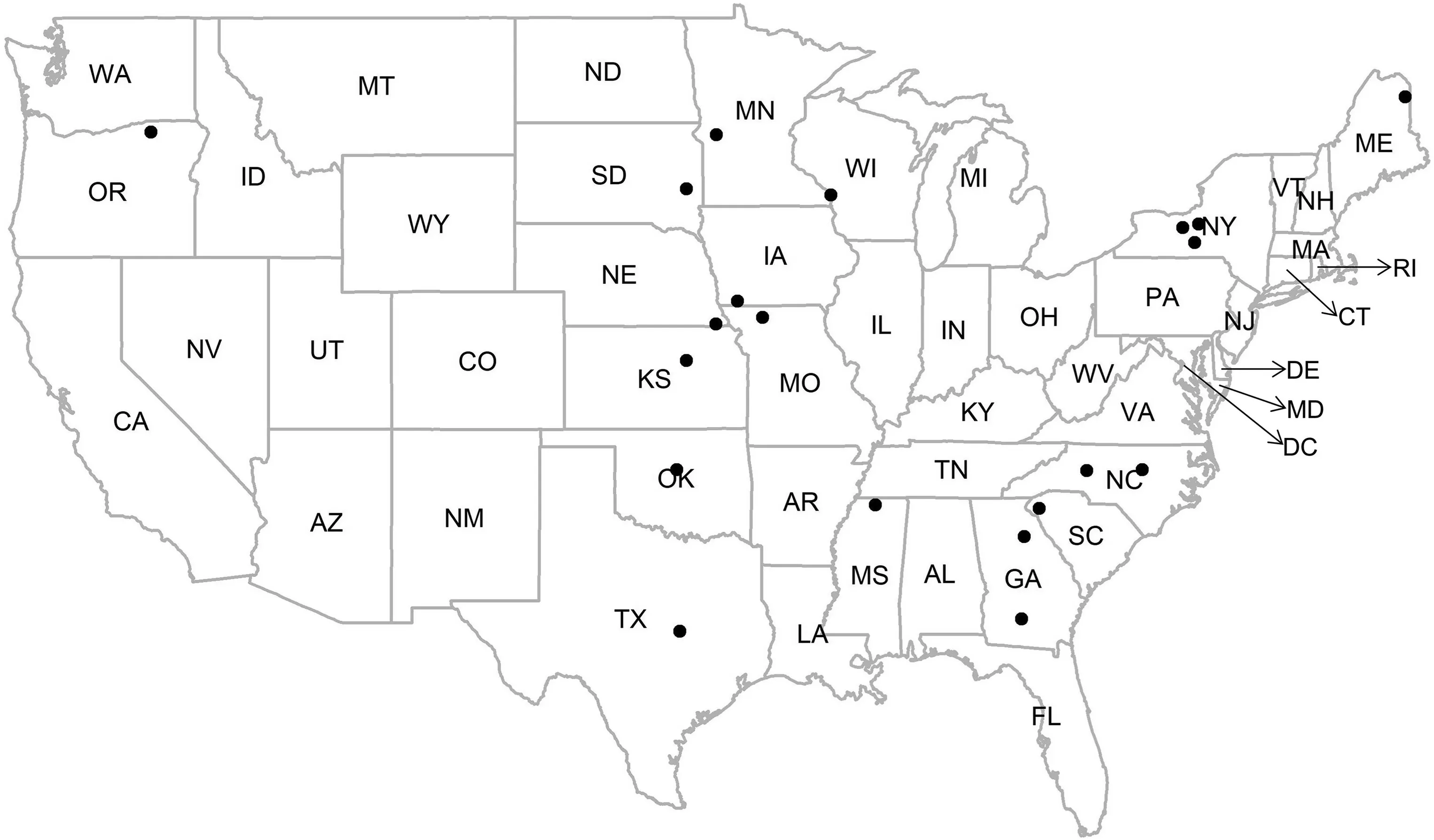
Fig.1.Field experimental plot locations in the USA in this study.

Table 1 Selected data from the USLE database for WEPP calibration, validation, and evaluation.

The topographic input files were created based on the erosion plot slope length,width,and shape.The soil texture and depth for each layer were used to generate the soil input files.Table 2 shows soil texture of the surface layer for all locations in the USLE and SSURGO (Soil Survey Geographic database).The SSURGO database contains the soil information collected by the National Cooperative Soil Survey over the course of a century.This database is available at https://websoilsurvey.sc.egov.usda.gov/App/WebSoilSurvey.aspx.For all locations considered in this study, the particle size distributions were comparable between the USLE database and the SSURGO database.For the other parameters in the soil input file,the baseline interrill erodibility (ki), baseline rill erodibility (kr), baseline critical shear stress (τc), and baseline effective hydraulic conductivity (ke) can be set to zero (0.0), which allowed these parameters to be calculated internally in WEPP (Flanagan and Livingston, 1995; Risse et al., 1994).For soils with sand content greater than 30%, these parameters were calculated using the equations in WEPP based on the fraction of very fine sand in Table 2.The method to calculate ke,kr,kiand τcwill be discussed later in this paper.Previous studies showed the WEPP model is sensitive to ke,kr,kiand τc(Brunner et al.,2004;Nearing et al.,1990;Pandey et al.,2008; Zheng et al., 2020).The determination of these parameters was inherently difficult and uncertain given there can be significant spatial variability.Therefore,these parameters were calibrated later in this study to improve model performance.

The management input file contains the information for plant physical properties and growth, residue properties and decomposition,tillage operations,residue management,contour conditions,crop rotations, and all relevant dates.The crop types, tillage operations,and crop yields were available in the USLE database.For crop growth parameters, the biomass energy ratio, harvest index, and the optimum yield under no stress conditions were calibrated to match the plot crop yield observations.All the other crop growth parameters were assumed the same as the values from the WEPP default database (Flanagan and Livingston,1995).

2.3.Calibration method

Four parameters were calibrated in this study to improve WEPP performance including baseline effective hydraulic conductivity(ke), baseline rill erodibility (kr), baseline critical shear stress (τc),and baseline interrill erodibility (ki).The selected parameters and procedures were consistent with Flanagan et al.(2012) and Risse et al.(1994).These parameters were calibrated to obtain the greatest Nash-Sutcliffe model efficiency(NSE)values for the runoff and soil loss predictions.Given the lack of data for soil depth to a restrictive layer,the soil depth factor was not considered for model calibration in this study.For plots with conservation tillage and notill, soil depth to a restrictive layer plays a vital role to distinguish the infiltration-excess and saturation-excess runoff events (Boll et al., 2015).In this study, all plots considered were with conventional tillage, especially tilled fallow plots, where runoff events were mainly infiltration-excess driven.Therefore, the calibration did not contain the soil depth factor.

Sensitivity analysis was conducted for the calibration of the WEPP model.The sensitivity ratio (SR) of a parameter can be calculated through Equation (1) (McCuen & Snyder,1986):

where Iminand Imaxare the minimum and maximum values of input used, Iaveis the average of Iminand Imax, Ominand Omaxare the corresponding outputs with Iminand Imaxinput values, and Oaveis the average of Ominand Omax.Sensitivity analysis can evaluate the relative magnitudes of changes in the model response to relative changes of model input parameters (Nearing et al., 1990).In the WEPP model, the soil erosion values were calculated based on the predicted runoff values.Therefore, the effective hydraulic conductivity parameter was calibrated first.The sensitivity ratio was then computed for the erosion parameters(baseline critical shear stress,baseline rill erodibility, and baseline interrill erodibility).Thecalibration of these parameters followed the order of sensitivity from the maximum to the minimum.

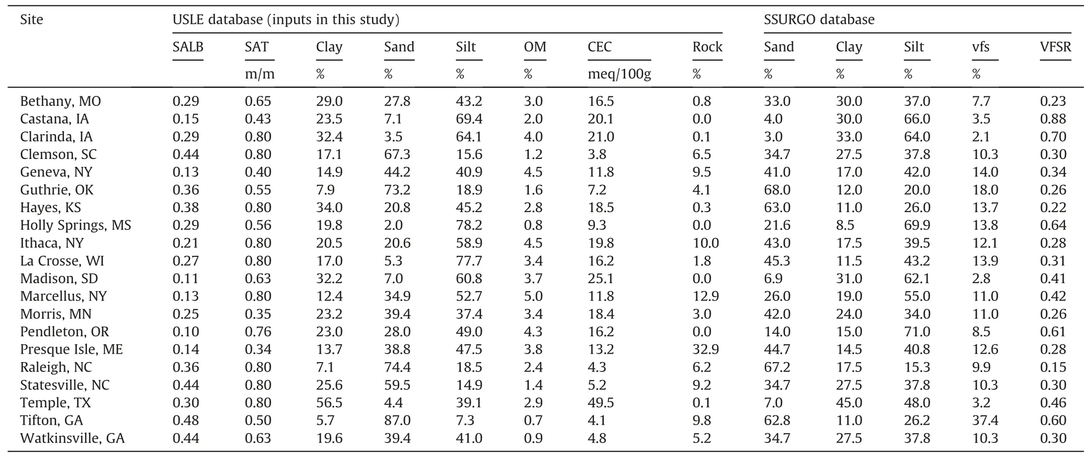
Table 2 Soil texture of the surface layer in the USLE database and the SSURGO database for all study locations.

In this study,the performance of the WEPP model was assessed without calibration first using all 1159 plot years of data in Table 1.The baseline effective hydraulic conductivity was calibrated with all 1159 plot years of data to obtain the best runoff predictions.On the basis of calibrated runoff,the baseline critical shear stress,baseline rill erodibility, and baseline interrill erodibility were calibrated through the same procedure with 607 plot years of data.The validation of WEPP calibrated soil loss predictions were then conducted using the rest of the 552 plot years of data.When dividing the data for calibration and validation, the data from earlier years were selected for calibration and the rest for validation for each experimental plot.If the plot had even years of records, the data were separated evenly for calibration and validation.Otherwise,the calibration dataset included one more year of records than the validation.

2.4.Data analysis

In this study, the WEPP model was applied with continuous long-term simulations for the total 134 plots (Table 1).The daily predictions of runoff and soil loss were selected for analysis from the model outputs.The event,monthly,annual,and average annual WEPP predictions were compared to the observations.Model performance was assessed using the coefficient of determination(R2),Nash-Sutcliffe efficiency (NSE), root mean square error (RMSE),percent bias (PBIAS), and absolute errors (mean, median, and standard deviation).The NSE indicates the agreement between the observed and predicted values (fit to the 1:1 line).Perfect agreement is reached with an NSE value of 1.Brooks et al.(2016) indicated that when using the daily output for streamflow prediction from an uncalibrated model,an NSE above 0.30 is a good indication that the fundamental mechanics of the model are correct.Foglia et al.(2009) considered NSE values below 0.2 insufficient,0.2-0.4 sufficient, 0.4-0.6 good, 0.6-0.8 very good, and greater than 0.8 excellent.The RMSE and the absolute errors describe the differences between predictions and observations.The R2indicates what proportion of the observed data can be explained by the model (Foglia et al., 2009; Moriasi et al., 2007).

The calibrated parameters (ke, τc, kr, and ki) were compared to the values obtained when using information from the Soil Survey Geographic database (SSURGO) and the calculations internally within the uncalibrated WEPP model.When using the uncalibrated WEPP model,the effective hydraulic conductivity is calculated with Equation (2) (Risse et al., 1994), and the baseline rill erodibility,baseline interrill erodibility, and baseline critical shear stress are calculated with Equations (3)-(5) (Alberts et al.,1995).

where ke(mm/h)is the baseline effective hydraulic conductivity,kr(s/m) is the baseline rill erodibility for cropland soils, τc(Pa) is baseline critical shear stress for cropland soils, ki(kg s/m4) is the baseline interrill erodibility for cropland soils,CEC(meq/100g)is the cation exchange capacity of the soil,clay is the fraction of clay in the surface soil,sand is the fraction of sand in the surface soil,vfs is the fraction of very fine sand in the surface soil, and orgmat is the fraction of organic matter in the surface soil.Given the vfs is not included in the soil input file but used to calculate kr, ki, and τcin Equations(3)-(5)for the surface soil with more than 30%sand,the vfs was obtained from the SSURGO database for the given type of soil.For the soil with very fine sand over 0.40(40%),the fraction of very fine sand was assumed to be 0.40 in Equations(3)-(5).In this study, ke, kr, ki, and τcwere calibrated to improve model performance.These calibrated parameters were compared to the ones calculated based on the particle size distributions of the SSURGO database and the USLE database with the vfs calculated in Equation(6):

where VFSR is the ratio of very fine sand in sand,vfssand sandsare the percentages of very fine sand and sand in the SSURGO database.For each location, the VFSR was calculated and shown in Table 2.Equation(6)assumes the VFSR for a given location is similar in the USLE database compared to the SSURGO database.

3.Results and discussion

3.1.Precipitation characteristics

Fig.2 reveals a large diversity in climate for the 20 sites considered in this study.The changes in annual precipitation among the study years are different at the various locations.In Watkinsville, GA, and Tifton, GA, the precipitation differences between wet years and dry years were over 800 mm for the time periods considered.In Raleigh, NC, Marcellus, NY, Madison, SD,Presque Isle, ME, and Pendleton, OR, the differences in annual precipitation were less than 300 mm.The greatest annual precipitation was recorded in Watkinsville,GA in 1964 as 1859.1 mm,and

Fig.2.Annual (a), average annual (b), and average monthly (c) precipitation depths for the sites in this study.

the lowest was in Hayes,KS in 1933 as 366.8 mm.Fig.2b shows the relatively dry areas were at Hayes,KS,Madison,SD,Pendleton,OR,and Morris,MN in this study with average annual precipitation less than 600 mm,and the relatively wet areas were at Watkinsville,GA,Holly Springs,MS,and Tifton,GA with average annual precipitation over 1200 mm.Fig.2c illustrates the average monthly precipitation for each location.Precipitation was centralized between June and September for most locations.There were some locations with precipitation concentrated early in the year(from February to May)including Clemson,SC,Temple,TX,Tifton,GA,and Watkinsville,GA.Rainfall and winter snowfall were the two main types of precipitation.Pendleton in Oregon had a significant snowfall amount in winter and relatively limited rainfall in summer.The average precipitation from June to August was only 72 mm in Pendleton, OR,which was about 12% of the average annual precipitation at this location.There were another five locations with large amounts of precipitation during the winter time including Holly Springs, MS,Statesville,NC,Temple,TX,Tifton,GA,and Watkinsville,GA.These locations are in the southern United States or near the east coast(Fig.1) with minimum temperatures greater than 0°C for most winter days.

Fig.3 shows the characteristics of average event precipitation intensity and average event intensity-at-peak factor(ip)for all sites considered in this study.Ip is the ratio of peak precipitation intensity to average precipitation intensity, which reflects the concentration level of the event.The sites in Fig.3 were sorted based on the average annual precipitation from the lowest to highest in Fig.2b.The site with great average event precipitation intensities(Fig.3a)means it has a large fraction of heavy events.In Fig.3b, lower average event ip means more relatively uniform precipitation events at that location.For the relatively wet sites with greater precipitation amounts,most of them also had greater fractions of heavy precipitation events and more concentrated events,such as Watkinsville,GA,Holly Springs,MS,and Tifton,GA.Comparing to these locations, Clemson, SC, Statesville, NC, and Raleigh,NC were wetter locations with more uniform events given lower average event ip observed.A great portion of heavy events were obtained in Temple, TX where the average annual precipitation and the average event ip were not high.Hayes, KS was the driest site in this study with the lowest precipitation amount,where high intensity events occurred relatively more often.Pendleton, OR was relatively dry where most events were more concentrated(greater average event ip).The runoff generation was affected by both the precipitation amount and distribution.Overall,a wide variety of climates were considered in this study.

Fig.3.Average event precipitation intensity (a) and average event intensity-at-peak(ip) factor (b) for the sites in this study.

3.2.Evaluation of the uncalibrated WEPP model predictions

3.2.1.Evaluation of runoff depth predictions

Fig.4 presents the comparison of runoff depth between uncalibrated WEPP predictions and the experimental field observations for different time scales.The R2, NSE, RMSE, PBIAS, and absolute errors are shown in Table 3 to assess model performance.When using the uncalibrated WEPP model for estimation,both the runoff and soil loss predictions were acceptable.For event model simulations, uncalibrated runoff predictions had a coefficient of determination(R2)of 0.64 and NSE of 0.59,while when going to coarser time scales, R2reached 0.83 and NSE was 0.82 for average annual predictions [Table 3, Fig.4 (a)], indicating excellent model performance and correct parameterization.The uncalibrated WEPP model tended to underestimate the average annual runoff for the plots with greater observations (greater than 200 mm).The plot with the greatest observed average annual runoff(315.7 mm)was a tilled fallow plot in Holly Springs,MS.The three greatest observed average annual runoff values were all recorded from tilled fallow plots.The three lowest observations were measured from plots in Geneva,NY,Ithaca,NY,and La Crosse,WI,and had continuous grass growing.The greatest difference between observed and predicted runoff was in a tilled fallow plot in Clemson, SC, with average annual runoff underestimated by 130.5 mm, followed by a tilled fallow plot in Holly Springs, MS, and another tilled fallow plot in Clemson, SC.

The uncalibrated WEPP model gave very good performance for prediction of annual [Fig.4 (b)] and monthly [Fig.4 (c)] runoff depths.The R2and NSE values reached 0.79 and 0.79 for annual runoff,and 0.70 and 0.70 for monthly runoff(Table 3).The tendency to underestimate annual runoff over 300 mm and monthly runoff over 150 mm was observed, which was similar to the average annual results.Most of the runoff overestimations were for Temple,TX,for all considered time scales.The soil type in Temple,TX is an Austin silty clay soil,and there were two types of cropping systems:continuous corn, and a corn-oats-cotton-rye rotation (Table 1).Fig.5 shows the average annual runoff predictions with the uncalibrated WEPP model for different soil types and slope gradients.There were eight different soil types considered in this study.The uncalibrated WEPP model tended to overestimate the average annual runoff for the silty clay and silty clay loam soils and underestimate for the sandy loam and loamy sand soils.When considering the uncalibrated WEPP performance for different slope gradients,no clear tendency was obtained and good average annual runoff predictions were observed for all considered slope gradients in this study.Table 4 shows the statistical analysis of event runoff predictions for all considered soils with the uncalibrated WEPP model.Good event runoff predictions were obtained for most of the soils considered in this study with NSE over 0.50 except for the silty clay loam(NSE=0.37)and the loam(NSE=0.22).When examining the observations in Fig.5, the event runoff tended to be overestimated for the silty clay(PBIAS=42.50%)and the silty clay loam(PBIAS=12.40%)and underestimated for the sandy loam(-42.10%)and loamy sand(-16.10%)soil types.For these four types of soil,the silty clay loam soils were located in Madison,SD and Clarinda,IA in this study.Given relatively small average annual precipitation[Fig.2 (b)] at these two locations with moderate average event precipitation intensities(4.6 mm/h and 4.5 mm/h in Fig.3(a),lower runoff would be expected, and Table 4 shows smaller mean absolute errors for runoff predictions.Greatest mean absolute errors were obtained for the Clemson, SC and Raleigh, NC locations with the sandy loam soils and relatively greater precipitation.Given the predicted runoff is used for soil loss predictions in WEPP, the calibration of the soil-related hydrology parameter(ke)was needed for some soil textures(e.g.,silty clay,silty clay loam and sandy loam)to improve model performance.

The event performance [Fig.4 (d)] shows a larger discrepancy between observations and predictions compared to the other time scales.The larger events with runoff over 100 mm tended to be overestimated.The underestimation of the average annual runoff in the two fallow plots in Clemson, SC [Fig.4 (a)] was mainly due to three events at this location.The underestimation outliers in Clemson,SC are shown in Fig.4(d).These events occurred on 7/17/1940, 8/12/1940, and 8/29/1940 with rainfall depths of 113.8 mm,145.3 mm, and 116.8 mm in 1.83 h,16 h, and 12 h, respectively.In Clemson,SC,the uncalibrated WEPP model tended to underpredict the event runoff in fallow plots for large events including two long duration ones (12 h and 16 h) and a single short duration one(1.83 h).This finding agreed with Zheng et al.(2020) that WEPP tended to underpredict runoff for extreme storms in the experimental plots with four different crops.The runoff depths were mostly overestimated in Temple, TX with silty clay soil.

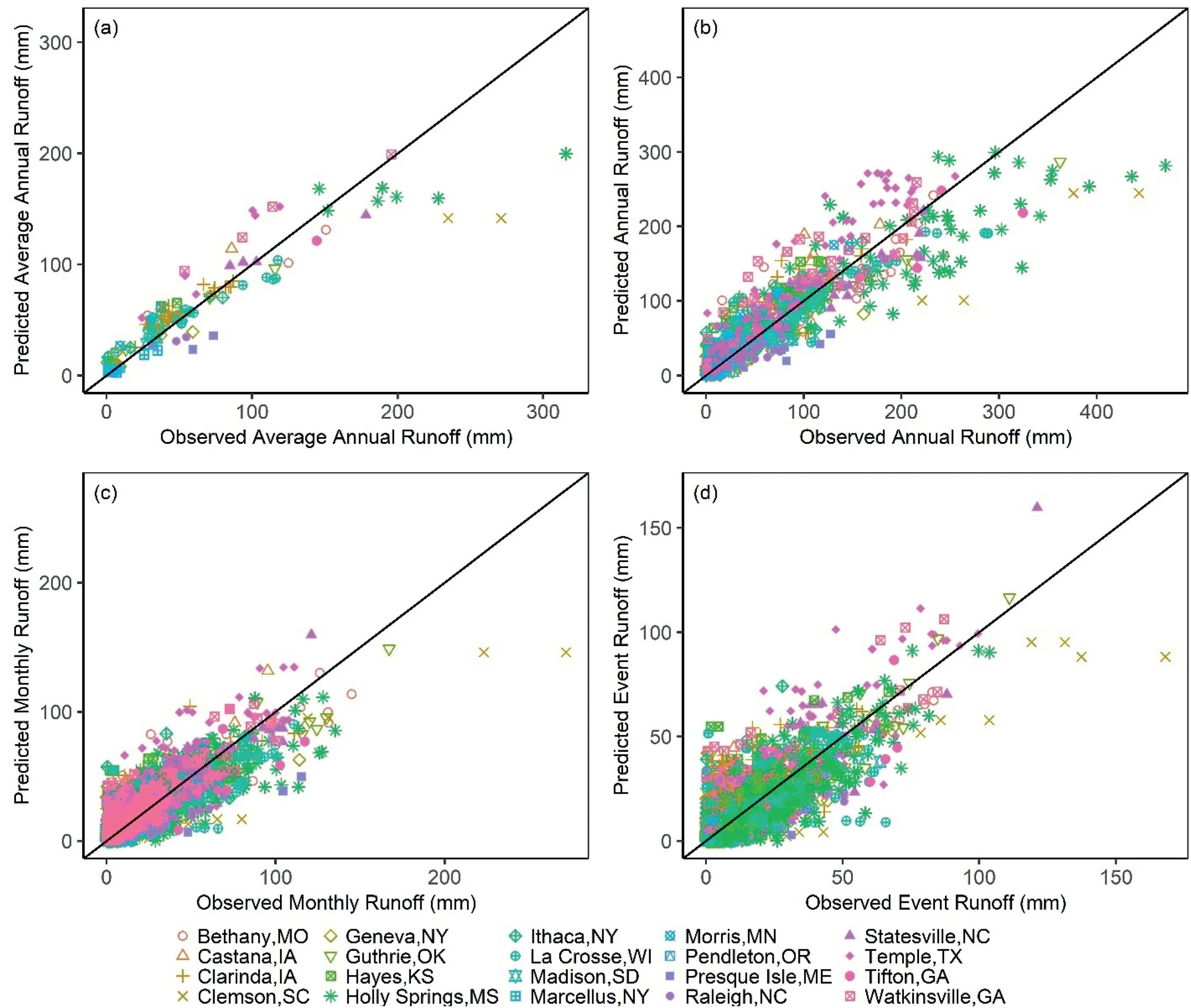
Fig.4.Observations and the uncalibrated WEPP predictions of average annual (a), annual (b), monthly (c), and event (d) runoff depths for the study sites.

Table 3 Statistical analysis results for WEPP model predictions.

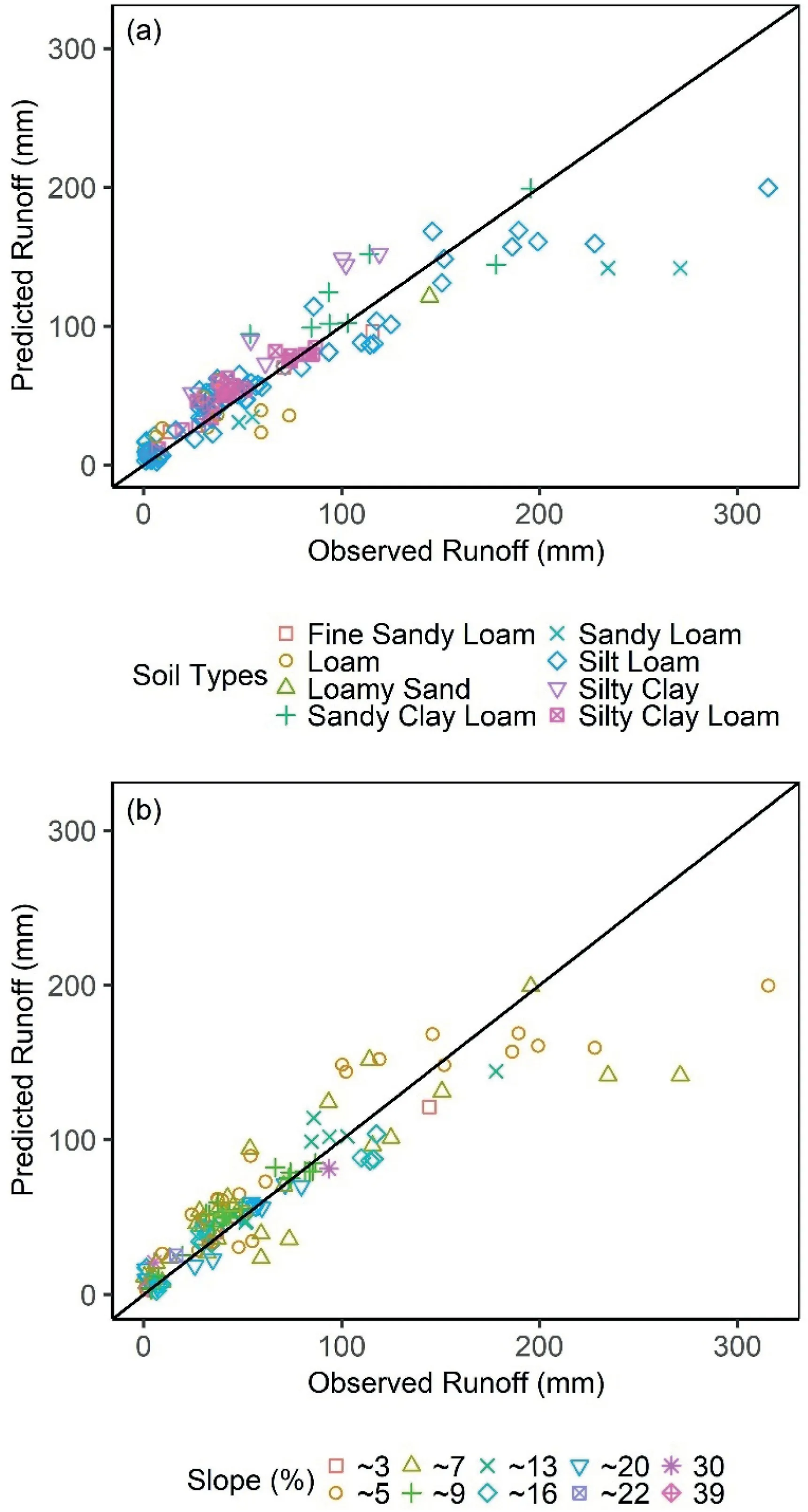
Fig.5.Observations and the uncalibrated WEPP predictions of average annual runoff depths for the different soil types (a) and slope gradients (b).

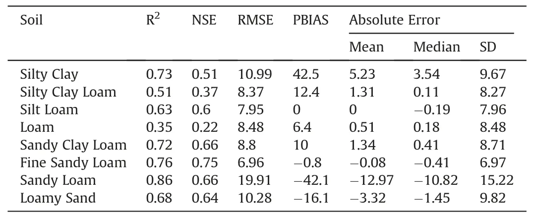
Table 4 Statistical analysis of event runoff predictions with the uncalibrated WEPP model.

3.2.2.Evaluation of soil loss predictions

Fig.6 presents the uncalibrated WEPP model performance for soil loss at different time scales.The left-side plots are linear graphs,which highlight the uncalibrated WEPP model performance for large soil loss events.The right-side plots are logarithmic graphs for soil loss values less than 100 t/ha to show the details of small events.The average annual comparison [Fig.6 (a)] indicates that good soil loss predictions were obtained when using the uncalibrated WEPP model (R2= 0.81, NSE = 0.72; Table 3).However,about two-thirds of the field plots had underestimated average annual soil loss and overall PBIAS was-38.6%.As we know,soil loss can increase exponentially as runoff increases (Wang et al., 2019;Zhang et al.,2009).The tendency to underpredict runoff for larger events may partially explain the underpredictions of soil loss.For the plots with average annual soil loss less than 1 t/ha, soil loss values for 17 of 21 plots were overpredicted[Fig.6(a)].All of these 21 plots had grass or rye crops.Given limited soil loss from these high cover crops, the greater relative errors between predictions and observations present small absolute errors which may be the result of one or two events.Nearing(1998)also explained why soil erosion models tend to underestimate larger soil loss events, and overpredict smaller events.

The field erosion plots with the greatest average annual soil losses(over 200 t/ha)were all at La Crosse,WI,with relatively steep slope gradients(16%for the tilled fallow plots and 30%for the corn plots).Among them,the greatest measured average annual soil loss was from a tilled fallow plot with a 16%slope gradient(368.8 t/ha).The two plots with the greatest differences between measurements and model predictions were tilled fallow ones in La Crosse,WI and Bethany, MO, with average annual soil loss underestimated by 116.1 t/ha and 99.2 t/ha,respectively.Fig.7 shows the event runoff and soil loss for these two continuous tilled fallow plots.Relatively good event runoff predictions were obtained with the uncalibrated WEPP model with NSE of 0.81 and 0.79 for these two locations.However, the soil loss was mainly underpredicted with PBIAS of -33.9% and -67.7%.For all the continuous tilled fallow plots considered in this study, there were 16 out of the 20 plots with underestimated average annual soil loss.Among these 16 plots,there were 10 plots with corresponding underestimated average annual runoff.Table 5 shows the statistical analysis of event runoff and soil loss for different crops.Before calibration, good runoff predictions were obtained for tilled fallow with NSE of 0.70,but the corresponding soil loss was underestimated with NSE of 0.45 and PBIAS of -42.9%.Therefore, the uncalibrated WEPP model tended to underestimate the soil loss of the continuous tilled fallow plots in this study, even though the runoff amounts were well predicted.Given that the sensitivity to soil-related parameters was greater for the tilled fallow plots,the unsatisfactory predictions may have been due to unsuitable soil-related baseline erodibility parameters(kr,τc,and ki) when using the uncalibrated WEPP model.

The uncalibrated WEPP model tended to underestimate soil loss for larger events (over 120 t/ha) and overestimate soil loss for smaller events (less than 0.01 t/ha) in Fig.6 (d).The monthly soil loss in Fig.6(c) was the accumulation of event soil loss for each month, which showed the tendency of underestimated values for monthly soil loss over 170 t/ha.Similar results were also obtained in previous studies (Kinnell, 2003; Tiwari et al., 2000; Zhang et al.,1996).The tendency to overpredict smaller events and underpredict larger events for both runoff and soil erosion is common in most soil erosion models (Nearing,1998; Tiwari et al., 2000).

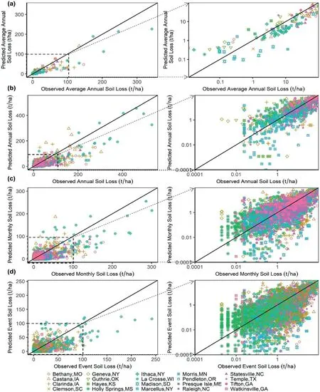
Fig.6.Observations and uncalibrated WEPP model predictions of average annual (a), annual (b), monthly (c), and event (d) soil loss for different sites.Left-side figures are linear plots for all soil loss values, while right side figures are logarithmic plots for soil loss values less than 100 t/ha.

3.3.Evaluation of calibrated WEPP predictions

3.3.1.Parameter calibration

The baseline effective hydraulic conductivity was first calibrated for the improvement of runoff prediction, given that soil loss is simulated as a function of runoff values in WEPP.The baseline hydraulic conductivity is defined as the maximum infiltration rate(mm/h), and the effective hydraulic conductivity for a given condition is adjusted to account for the effects of canopy cover and residue on the basis of the baseline value (Risse et al.,1995).The baseline effective hydraulic conductivity was calibrated for each experimental field plot with the entire dataset (1159 plot years),and the test range for this parameter was 0.07-10.0 mm/h(Table 6), which is the same range as in Risse et al.(1994).A sensitivity analysis was conducted for the baseline rill erodibility,baseline interrill erodibility, and baseline critical shear stress with the test ranges shown in Table 6 for each parameter.The test ranges for these parameters were similar to the ranges in Nearing et al.(1990).The sensitivity analysis indicated that the baseline critical shear stress was the most sensitive parameter with greatest absolute SR of 0.512 in this study,followed by the baseline rill erodibility and the baseline interrill erodibility, without consideration of the effective hydraulic conductivity.These parameters were then calibrated for each location following the order of the absolute SR value from largest to smallest: baseline critical shear stress, baseline rill erodibility, and baseline interrill erodibility.For each location,about half of the records for all plots were used for calibration.The entire calibration dataset contained 607 plot years of records.

Fig.7.Observations and the uncalibrated WEPP model predictions of event runoff and soil loss for the tilled fallow plots at Lacrosse, WI (a) and Bethany, MO (b).

Table 5 Statistical analysis results of the event runoff and soil loss for different crops.

Fig.8 shows the comparison of calibrated parameters to the values based on the SSURGO database and the USLE database for alllocations(Table 2).The USLE parameterized values were calculated based on equations(2)-(5),which were the default values in WEPP without calibration.The results indicated reasonable calibrated values were obtained for the four parameters,given that the values were comparable to the ones based on the SSURGO database or the USLE database.For these four parameters, the optimum values through calibration were either close to the corresponding values in SSURGO or USLE, or in the range between these two resources.Given the surface soil texture can be different more or less for a given location,the parameters considered were calibrated for each experimental plot.For most locations considered in this study,the calibrated parameters for one location were within a small range,which agreed with similar surface soil textures for all plots at a given location.For some locations in Fig.8, the differences were greater between the USLE and the SSURGO parameterizations compared to the other locations, including the baseline effective hydraulic conductivity in Hayes, KS, the baseline critical shear stress in La Crosse,WI,the baseline rill erodibility in Holly Springs,MS,and the baseline interrill erodibility in Tifton,GA.Differences at these locations were caused by the differences of the soil texture recorded in the USLE database and the SSURGO database(Table 2).The relatively greater differences of surface soil texture between the USLE database and the SSURGO database may support larger discrepancies at these locations.

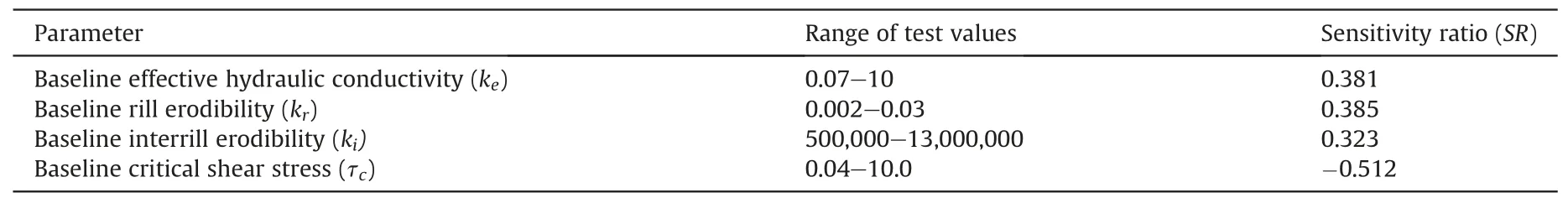
Table 6 Sensitivity ratios(SR) for the baseline effective hydraulic conductivity, rill erodibility, interrill erodibility, and critical shear stress.

Fig.9.Comparisons between uncalibrated and calibrated baseline effective hydraulic conductivity (a), baseline critical shear stress (b), baseline rill erodibility (c), and baseline interrill erodibility (d).(Note: ke is baseline effective hydraulic conductivity, τc is baseline critical shear stress, kr is baseline rill erodibility, and ki is baseline interrill erodibility.)

Fig.9 shows the comparisons between uncalibrated and calibrated baseline effective hydraulic conductivity, baseline critical shear stress, baseline rill erodibility, and baseline interrill erodibility.Given the plots at the same site had similar characteristics,for some sites and some parameters,the calibrated values were the same for several plots.Therefore,some scatter points overlapped in the subplots in Fig.9, and each subplot shows the comparison for 134 plots considered in this study.The uncalibrated and calibrated values of these four parameters are provided in appendix A for each plot.In Fig.9 (a), the calibrated baseline kevalues tended to be greater than the uncalibrated values for the plots with lower keand smaller than the uncalibrated values for larger keplots.The tendency of greater calibrated than uncalibrated kewas obtained for silty clay and silt loam soils,and the opposite trend was discovered for sandy clay loam, fine sandy loam, and loamy sand.The calibrated kevalues were greater than the corresponding uncalibrated kevalues for almost all tilled fallow plots(Appendix A).The results for the tilled fallow plots indicated that the general parameterization equations may not be sufficient to describe some soil types,which may then need calibration to improve WEPP model predictions.For τc, kr, and kiin Fig.9 (a), (b), and (c), the calibrated values and uncalibrated values were relatively uniformly distributed around the 1:1 line for all soils considered in this study.

3.3.2.Evaluation of runoff depth predictions

Fig.10 and Table 3 present WEPP model performance for runoff predictions after the calibration of effective hydraulic conductivity.The predictions for all considered times scales were improved through this calibration.The NSE values increased from 0.82,0.79,070, and 0.59 to 0.98, 0.91, 0.81, and 0.70 for average annual,annual, monthly, and event runoff depth predictions, respectively(Table 3), through calibration.The PBIAS values were very close to the optimum 0.0% for all time scales considered.Good runoff predictions for large storms were obtained through the calibration.After calibration,the plot having the greatest difference in average annual runoff was a corn-Bermuda grass rotation plot at Watkinsville,GA,with a difference of 37.8 mm[Fig.10(a)],which was much less than the greatest difference of 130.5 mm at Clemson,SC,before calibration.

Fig.10 (d) shows good agreements between predicted and observed event runoff depths after calibration.The greatest difference was 54.3 mm at Temple,TX which was less than the single event difference of 81.2 mm at Clemson,SC before calibration.The greatest discrepancies were at Temple, TX with 2 outlier events,which occurred on 4/21/1945 and 9/7/1942 at the continuous corn and corn-oats-cotton-rye rotation plots, respectively.The rainfall depths on 4/21/1945 and 9/7/1942 were 129.5 mm and 141.5 mm in 10.2 h and 17.0 h, respectively.These two events occurred on relatively bare soil surfaces when the corn was not planted yet or the cotton was just harvested.Given greater sensitivity to the soilrelated parameters, the runoff predictions for large rainfall events on bare soil were more challenging in most cases.Meanwhile, the WEPP model tended to overestimate runoff from silty clay soils(Fig.5), which may also have contributed to the overpredicted runoff at Temple, TX.

3.3.3.Evaluation of soil loss predictions

The calibrations of the erosion-related parameters(τc,kr,and ki)were based on simulations using about half of the data (607 plot years).Table 3 shows WEPP soil loss prediction performance improved for the calibration data (607 plot years), the validation data (552 plot years), and the entire dataset (1159 plot years).The WEPP model performance for the entire dataset improved from NSE of 0.72,0.63,0.56,0.49 to 0.91,0.78,0.69,0.63 for the average annual, annual, monthly, and event soil loss predictions (Table 3),respectively.Good soil loss predictions were obtained for all time scales considered given the NSE values were all over 0.6.Also, the PBIAS improved from -38.60% to -25.10% for the average annual scale and improved from -38.20% to -26.80% for the annual,monthly, and event scales.Fig.11 shows the calibrated WEPP performances for soil loss predictions for all time scales considered.The predictions were improved for both the calibration dataset and the validation dataset(Table 3).The NSE of average annual soil loss improved from 0.59 to 0.89 for the calibration dataset and improved from 0.71 to 0.85 for the validation dataset.Given that WEPP soil loss is computed based on simulated runoff, one would expect model performance for soil loss predictions to be somewhat lower than those for runoff prediction.

Fig.11 shows the performance of the calibrated WEPP model for different scales.The greatest difference between event predicted and observed soil loss was at La Crosse,WI in the validation dataset[Fig.11 (d)].The difference was 95.6 t/ha, which was less than the 130.1 t/ha before calibration.Also at La Crosse,the soil loss tended to be underestimated for the larger events and overestimated for the smaller events for the validation dataset.Model validation was impacted by the selection of the calibration and validation data,especially at La Crosse,where the greatest observed soil loss in the calibration dataset was 71.5 t/ha lower than the greatest value in the validation dataset.Fig.11 shows that more large observed erosion events were included in the validation data having soil loss over 150 t/ha, especially for La Crosse, WI.Therefore, soil loss predictions for larger events at La Crosse were poorer for the validation dataset compared to the calibration dataset, as the calibrated model input parameters were all based upon lesser soil loss values.

3.4.WEPP performance for different crops and crop rotations

Table 5 shows the results of the statistical analysis of the event runoff and soil loss for different cropping/management systems.All considered crops were summarized as 10 classes.The hay crops class included alfalfa, bromegrass, Bermuda grass, and clover.Before calibration, there were 5 of the 10 crops with good runoff predictions (NSE ≥0.4) including corn, cotton, tilled fallow, oats,and soybeans.The event runoff depth was overestimated by about 50% for the plots with wheat, resulting in the low NSE of 0.03 in Table 5.The wheat considered in this study was winter wheat at Guthrie, OK and Hayes, KS.The overall overestimation of runoff depth was caused by model overpredictions for almost all events in the early spring.At this time, the surface cover was relatively limited and a small absolute error in surface cover could cause a large error in runoff predictions, which may be the reason for wheat runoff overestimations in Table 5.Lowest NSE values were obtained from rye and potato crop plots.Similar to the wheat plots considered in this study,most of the rye plots were winter rye with most event runoff overestimated in the early spring.When using the uncalibrated WEPP model for winter crop growth predictions,it seems that there was not sufficient crop biomass and cover information when only crop yield inputs were available and WEPP default values were used,especially for the early spring events.The crops with the least amount of plant growth data were potato and tobacco in this study and the model efficiencies were greatly affected by one or two outliers for these two crops.The greatest PBIAS was obtained for hay crops (60.80%); however, the mean absolute event error was as low as 3.19 mm.This is because the runoff depths were relatively small for the sod cropped plots and the small absolute error could result in large relative errors for these predictions.

The event runoff predictions were improved for all crop/management systems through calibration.There were 8 of 10 crops with good event runoff predictions (NSE ≥0.4) after calibration including corn,cotton,tilled fallow,oats,potato,soybeans,tobacco,and wheat.The greatest PBIAS was obtained for hay crops as 33.50%, which was an improvement from the 60.80% before calibration.Also, the mean absolute error was 2.04 mm for hay crop event runoff predictions.The mean absolute errors of runoff depth were under 2.70 mm for all considered crops after calibration.The best event runoff predictions were obtained in tilled fallow plots both before and after calibration.

Fig.11.Observations and the calibrated WEPP model predictions of (a) average annual, (b) annual, (c) monthly, and (d) event soil loss for the different sites.

Given that the soil loss predictions in the WEPP model were obtained on the basis of the predicted runoff depth,the NSE values for soil loss were lower than those for runoff for almost all crops as expected (Table 5).For cropping systems with good runoff predictions(NSE ≥0.4)before calibration,there were three with good soil loss predictions(NSE ≥0.4),which were corn,cotton,and tilled fallow with NSE of 0.45, 0.51, and 0.45, respectively.After calibration,for cropping systems with good runoff predictions,there were 4 of 8 with good soil loss predictions including corn, cotton, tilled fallow, and wheat.The lowest NSE values were obtained for oats,potato, and rye.Oats and potato were two crops with limited soil loss.The greatest observed event soil loss for oats and potato plots were 30.4 and 5.4 t/ha, respectively, which were quite low compared to the greatest event soil losses of 242.2, 132.2, and 94.7 t/ha for tilled fallow, corn, and cotton plots, respectively.Observed soil losses from soybean plots were also low (greatest observation was 12.2 t/ha).For crops having limited soil loss, a small absolute difference could appear as a large relative difference and generate poor NSE values.After calibration,the mean absolute errors of event soil loss were less than 2.80 t/ha for all considered crops.For the common cropping systems, model efficiency (NSE)values were 0.64 for corn,0.58 for cotton,0.63 for tilled fallow,0.45 for wheat, and 0.33 for soybeans.

Given the lack of daily maximum and minimum temperatures,dew point temperature, wind speed and direction, and solar radiation in this study, CLIGEN was used for the simulation of these parameters.All these weather factors affect the predictions of crop growth, evapotranspiration (ET), soil moisture, and water balance in the WEPP model.Even though some of the crop growth parameters (the biomass energy ratio, harvest index, and the optimum yield under no stress condition)were calibrated based on the observed crop yields, the use of partially simulated climate inputs can cause errors in daily crop growth and water balance predictions and then lead to errors in the subsequent daily runoff and soil loss predictions.Therefore, better runoff and soil loss estimations can be expected through WEPP when detailed climate input parameters are available including precipitation amount, duration, and intensity, daily maximum and minimum temperatures, dew point temperature, wind speed and direction, and solar radiation.

4.Conclusions

This study evaluated the applicability of the WEPP model for runoff and soil loss predictions with a portion of the USLE database including 1159 plot years of rainfall-runoff data.The performance of WEPP model predictions were analyzed before and after calibration of the baseline effective hydraulic conductivity, baseline critical shear stress, baseline rill erodibility, and baseline interrill erodibility.Satisfactory predictions of both runoff and soil loss were obtained when using an uncalibrated WEPP model, with model efficiency (NSE) values of 0.82 and 0.72 for average annual estimates, respectively.After calibration,the predictions of runoff and soil loss were both improved with NSE values of 0.98 and 0.91,respectively.The calibrated parameters (ke, τc, kr, and ki) for each location were comparable to the values calculated based on the SSURGO database and the USLE database.The uncalibrated WEPP model tended to underestimate the runoff for large events with observed runoff over 100 mm.This tendency disappeared after the calibration of the baseline effective hydraulic conductivity.Both the uncalibrated and calibrated WEPP model tended to underestimate the soil loss amounts for large events with over 120 t/ha soil loss.There were 10 different cropping systems considered in this study.Before calibration, event runoff predictions were good (NSE ≥0.4)for most of the common ones, including corn, cotton,tilled fallow,oats, and soybeans.Corn, cotton, and tilled fallow systems all had good event runoff and soil loss predictions before calibration.After calibration,the model efficiency improved for all considered crops,and corn, cotton, tilled fallow, and wheat systems had good event runoff and soil loss predictions.For a more comprehensive evaluation of the WEPP model, future research could estimate WEPP performance for snowmelt-runoff events.Given the database used in this study was collected in 1931-1980 with a lack of modern cropping systems and tillage practices, future examination with available data could,for instance,investigate the WEPP runoff and soil loss predictions for conservation tillage and no-till with the calibration of soil depths and the depth to a restrictive layer.

Declaration of competing interest

The authors declare that they have no known competing financial interests or personal relationships that could have appeared to influence the work reported in this paper.

Acknowledgements

Funding supporting this research was provided by the USDANatural Resources Conservation Service (ARS-NRCS Interagency Agreement #60-5020-8-003) through the USDA-Agricultural Research Service and the Purdue University Department of Agricultural&Biological Engineering.The natural runoff plot data was provided by the USDA-Agricultural Research Service, National Soil Erosion Research Laboratory.

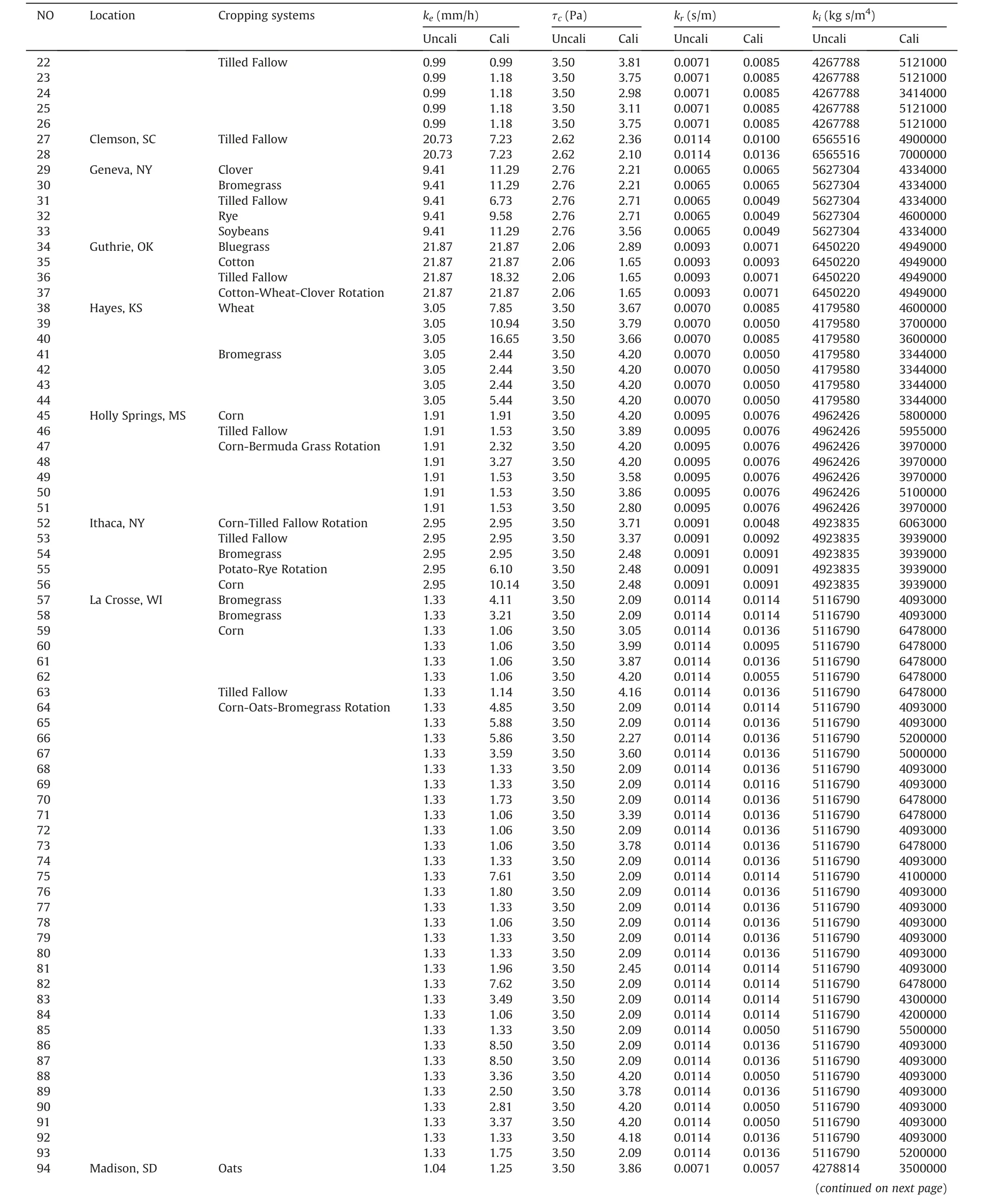
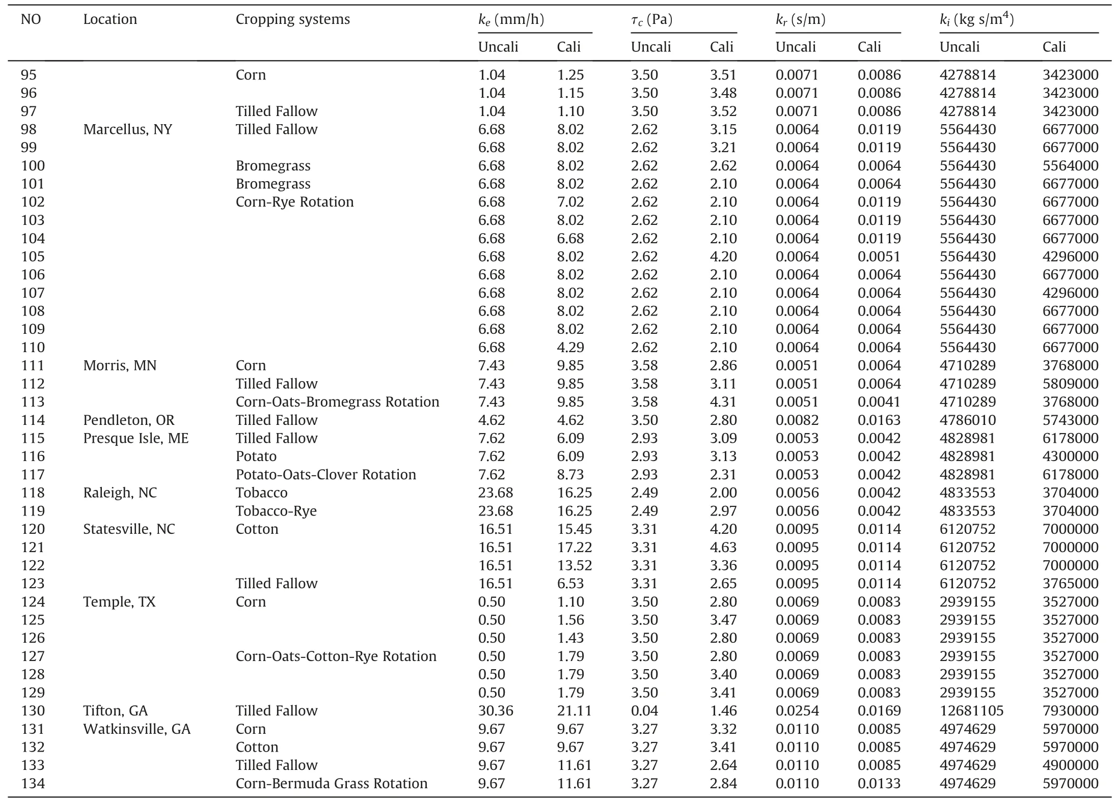
Appendix A

?NO Location Cropping systems ke (mm/h) τc (Pa) kr (s/m) ki(kg s/m4)Uncali Cali Uncali Cali Uncali Cali Uncali Cali 1 Bethany, MO Alfalfa 4.55 6.24 3.50 4.60 0.0073 0.0035 4455230 3366000 2 Bluegrass 4.55 6.95 3.50 2.80 0.0073 0.0073 4455230 3366000 3 Corn 4.55 3.64 3.50 3.12 0.0073 0.0088 4455230 3366000 4 Tilled Fallow 4.55 3.64 3.50 3.49 0.0073 0.0088 4455230 3366000 5 Castana, IA Tilled Fallow 1.24 1.48 3.50 3.84 0.0081 0.0073 4758445 5710000 6 Clarinda, IA Alfalfa-Corn Rotation 0.99 1.18 3.50 2.80 0.0071 0.0085 4267788 5121000 7 Corn-Bromegrass Rotation 0.99 0.99 3.50 2.80 0.0071 0.0071 4267788 5121000 8 Corn 0.99 0.99 3.50 2.88 0.0071 0.0085 4267788 3414000 9 0.99 1.18 3.50 4.20 0.0071 0.0085 4267788 5121000 10 0.99 0.99 3.50 3.28 0.0071 0.0085 4267788 3500000 11 Corn-Oats-Bromegrass Rotation 0.99 1.18 3.50 3.56 0.0071 0.0085 4267788 4900000 12 0.99 1.18 3.50 2.80 0.0071 0.0085 4267788 3414000 13 0.99 1.18 3.50 4.20 0.0071 0.0057 4267788 5121000 14 Corn 0.99 1.18 3.50 3.75 0.0071 0.0085 4267788 5121000 15 0.99 1.18 3.50 3.75 0.0071 0.0085 4267788 5121000 16 0.99 1.18 3.50 2.80 0.0071 0.0057 4267788 5121000 17 0.99 1.18 3.50 3.74 0.0071 0.0085 4267788 5121000 18 0.99 1.18 3.50 3.74 0.0071 0.0085 4267788 5121000 19 Corn-Rye Rotation 0.99 1.18 3.50 2.80 0.0071 0.0057 4267788 3414000 20 0.99 1.18 3.50 2.80 0.0071 0.0057 4267788 3414000 21 0.99 1.18 3.50 2.80 0.0071 0.0057 4267788 3414000

(continued)

(continued)