Exact Boundary Controllability for a 1-D Second-Order Quasilinear Hyperbolic System

,-

(1. Department of Mathematics, Donghua University, Shanghai 201620, China; 2. Institute for Nonlinear Sciences, Donghua University, Shanghai 201620, China)

Abstract: In this paper, we propose a second-order quasilinear hyperbolic system.By means of the theory on semi-global C1 solution to first-order quasilinear hyperbolic systems, we establish the existence and uniqueness of semi-global C2 solution to this second-order quasilinear hyperbolic system.After then,the general constructive framework is utilized to obtain the local exact boundary controllability for this second-order system.

Keywords: First-order quasilinear hyperbolic system; Second-order quasilinear hyperbolic system; Semi-global solution; Exact boundary controllability

§1.Introduction

Hyperbolic equation is a classof extremely important partial differential equations.Rich research has been obtained from both theoretical and practical perspectives for first-order quasilinear hyperbolic systems.The local exact boundary controllability can be defined as follows: There exists a control timeT>0, for any arbitrarily given initial state and final state in a neighborhood of an equilibrium, by means of suitable boundary controls, the system can drive the initial state exactly to the final state.Results on the local exact boundary controllability for 1-D first-order quasilinear hyperbolic systems can be found in [2], [3], [5], [6], [13].However,second-order quasilinear hyperbolic systems are more difficult and challenging than first-order ones in terms of definition, theory and application.The 1-D quasilinear wave equation, as a single second-order quasilinear hyperbolic equation, has been deeply studied and widely applied in many fields such as mechanics, materials science, etc (see [1], [7]).In this paper, we propose a second-order quasilinear hyperbolic system, and obtain the semi-globalC2solution to this system by means of corresponding theory on first-order systems.In addition, constructive methods are utilized to study the local exact boundary controllability for this second-order quasilinear hyperbolic system.

The recent works on the local exact boundary controllability study some special second-order quasilinear hyperbolic systems.For instance, in [17], Zhuang and Shang studied a single 1-D second-order quasilinear hyperbolic equation in the form:

where (a2-4b)(0,0,0)>0 and the 1-D quasilinear wave equation is included as a particular case.They obtained the well-posedness and local exact boundary controllability for this system.They also established the local exact boundary observability for it in [9].

With regard to second-order quasilinear hyperbolic systems composed by more than one equations, on account of the complexity of the coupled matrix, there are few deep studies on the exact boundary controllability for this kind of systems.For the following second-order quasilinear hyperbolic system:

whereu=(u1,...,un)Tis the unknown vector function of (t,x), the coupled matrixApossesses only positive eigenvalues, Yu obtained its local exact boundary controllability in [14].Later, she studied the following second-order quasilinear hyperbolic system:

whereu=(u1,...,un)Tis the unknown vector function of (t,x), the coupled matricesAandBcontain only positive or negative eigenvalues, respectively.She established its controllability and observability in [15] and [16], respectively.

For the second-order quasilinear hyperbolic system in more general form:

whereu=(u1,...,un)Tis the unknown vector function of(t,x),AandBaren×nmatrices.One of the authors in this paper proposed a sufficient condition for the hyperbolicity of this system in[10],that is,the coupled matricesAandBsatisfyAB=BA,the well-posedness of semi-globalC2solution is discussed and the local exact boundary controllability and observability are obtained by means of the constructive method (see [11], [12]).

In this paper, we also consider the above general second-order quasilinear hyperbolic system(1.1) in the case where the coupled matricesAandBare the same type of triangular matrix.We establish the existence and uniqueness of the corresponding semi-global solution and study its local exact boundary controllability by the constructive method.

§2.A 1-D second-order quasilinear hyperbolic system

In this paper, we are concerned with the 1-D second-order quasilinear system (1.1) in which the coupled matricesAandBare both triangular matrices with the same type.Without loss of generality, we assume thatn=2 and

are both lower triangular matrices,αi,βi(i=1,2),a,bare allC1functions with respect to their arguments andC(u,ux,ut)=(c1,c2)TisC1vector function with

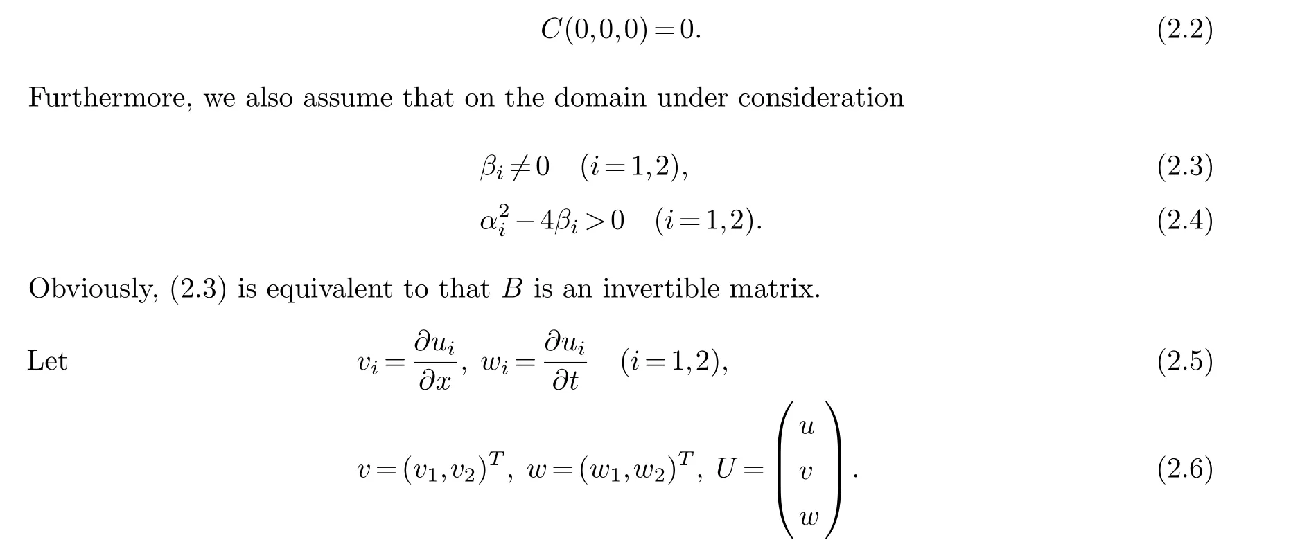
Then system (1.1) can be reduced to the following first-order quasilinear system

The characteristic equation of (2.7) is

SinceAandBare lower triangular matrices, det(λ2I2-λA+B)=0 can be rewritten as

Noting (2.4), it is easy to see that the first-order quasilinear system (2.7) possesses 6 real eigenvalues:

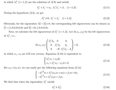
system (2.7) has a complete set of eigenvectors.

and it is easy to know that this is a complete set.Thus, the first-order system(2.7)is hyperbolic which implies that the system (1.1) under discussion is indeed a second-order quasilinear hyperbolic system.

Remark 2.1.The form of the second-order quasilinear hyperbolic system(1.1)considered in this paper is similar to that of in[10],but the requirements for the coupled matrices A and B are different,specifically,in our result,the coupled matrices A and B are both lower triangular matrices,which do not have to satisfy the condition AB=BA proposed in[10].

Remark 2.2.In this paper,we only discuss that u is a two-dimensional vector,while the method utilized here can be applied to the case when u is any dimensional vector.

§3.Existence and uniqueness of semi-global C2 solution

For the second-order quasilinear hyperbolic system (1.1) under consideration, we give the following initial condition

and final condition

where?=(?1,?2)Tand Φ=(Φ1,Φ2)Tare givenC2vector functions,ψ=(ψ1,ψ2)Tand Ψ=(Ψ1,Ψ2)Tare givenC1vector functions.

case(1)Inequality(3.3)is equivalent toβi<0.In this case,the number of positive eigenvalues and that of negative eigenvalues for system (1.1) are equal.For this case, we prescribe the following boundary conditions:

First of all, for case(1), we show the theorem on the existence and uniqueness of semi-globalC2solution to mixed initial-boundary problem (1.1), (3.1) and (3.6)-(3.7).

Theorem 3.1.Suppose that(2.3), (2.16)and(3.3)hold,and suppose furthermore that the conditions of C2compatibility are satisfied at the points(t,x)=(0,0)and(0,L),respectively.Then,for any given and possibly quite large T>0,the forward mixed initial-boundary value problem(1.1), (3.1)and(3.6)-(3.7)admits a unique semi-global C2solution u=u(t,x)on the domain R(T)={(t,x)|0≤t≤T,0≤x≤L} with small C2norm,provided that the norms‖(?,ψ)‖C2[0,L]×C1[0,L]and ‖(H,H)‖C2[0,T]×C2[0,T]are small enough.

Remark 3.1.The conditions of compatibility require that the initial data and boundary values be consistent and compatible with the given system.For the system(1.1)under consideration,let’s take the point(t,x)=(0,0)as an example.At this point,the conditions of C2compatibility would be:

In order to prove Theorem 3.1, we first review the well-posedness of semi-globalC1solution to first-order quasilinear hyperbolic systems (see Chapter 2 of [2]).

Lemma 3.1.Considering the following first-order quasilinear hyperbolic system:

where u=(u1,···,un)T,F(0)=0,matrix A has n real eigenvalues:

and a complete set of left eigenvectors li(u) (i=1,···,n).

Let

We give the following initial condition and boundary conditions for system(3.10)

where Gr(t,0,···,0)≡0,Gp(t,0,···,0)≡0.

Suppose that A,F,Gp,Gr,Hp and Hr(p=1,···,l;r=m+1,···,n)are C1functions with respect to their arguments,and suppose furthermore that the conditions of C1compatibility are satisfied at the points(t,x)=(0,0)and(0,L),respectively.Then,for any given and possibly quite large T>0,the forward mixed initial-boundary value problem(3.10)-(3.13)admits a unique semi-global C1solution u=u(t,x)on the domain R(T)={(t,x)|0≤t≤T, 0≤x≤L}with small C1norm,provided that the norms ‖φ‖C1[0,L],‖(Hp,Hr)‖C1[0,T]×C1[0,T]are small enough(p=1,...,l;r=m+1,...,n).

Now we give the proof of Theorem 3.1.

Proof.Let

By (2.17), we can get

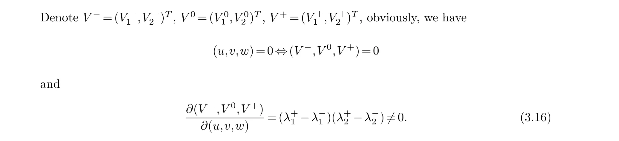
Hence, by the implicit function theorem, there existC1vector functions ～G=(～G1,～G2)Tand～H=(～H1, ～H2)Tin a neighborhood ofU=0, such that

and satisfy

Noting the conditions ofC2compatibility at the points (t,x)=(0,0) and (0,L), the initial condition (3.1) can be rewritten into

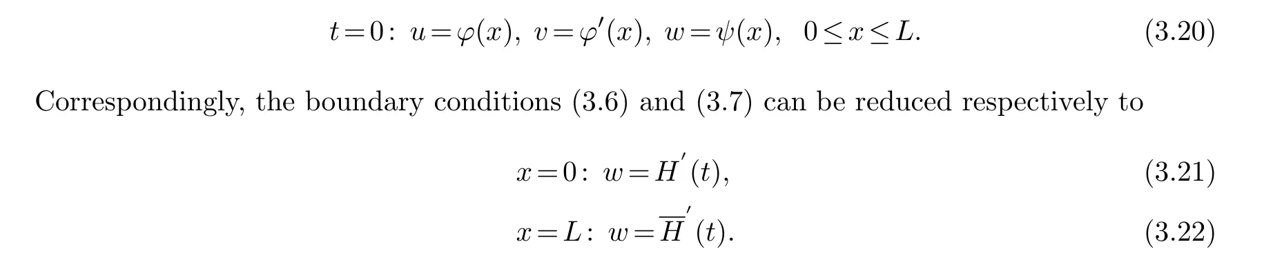
By (3.19), in a neighborhood of (u,v,w)=(0,0,0), the boundary condition (3.21) can be equivalently rewritten as

Moreover, it follows easily from the conditions ofC2compatibility of the original mixed initial-boundary value problem (1.1), (3.1) and (3.6)-(3.7) that the mixed initial-boundary value problem (2.7), (3.20) and (3.21)-(3.22) satisfies the conditions ofC1compatibility at the points(t,x)=(0,0)and(0,L), respectively.Then, by Lemma 3.1, system(2.7),(3.20)and(3.21)-(3.22)has a unique semi-globalC1solution, which implies that the original mixed initial-boundary value problem (1.1), (3.1) and (3.6)-(3.7) admits a unique semi-globalC2solution for case (1).The proof of Theorem 3.1 is complete.

Similarly,for the backward mixed initial-boundary value problem(1.1),(3.2)and(3.6)-(3.7),we can establish the well-posedness of the semi-globalC2solution.

Proposition 3.1.Suppose that(2.3), (2.16)and(3.3)hold.For any given and possibly quite large T>0,and for any given(Φ,Ψ), (H,H),suppose that the conditions of C2compatibility are satisfied at the points(t,x)=(T,0)and(T,L),respectively.The backward mixed initialboundary value problem(1.1), (3.2)and(3.6)-(3.7)admits a unique solution u=u(t,x)on the domain R(T)={(t,x)|0≤t≤T, 0≤x≤L} with small C2norm,provided that the norms‖(Φ,Ψ)‖C2[0,L]×C1[0,L]and ‖(H,H)‖C2[0,T]×C2[0,T]are small enough.

For case (2), we can obtain the existence and uniqueness of semi-globalC2solution in the same way.

Theorem 3.2.Suppose that(2.3)-(2.4), (2.16)and(3.4)hold,and suppose furthermore that the conditions of C2compatibility are satisfied at the point(t,x)=(0,0).Then,for any given and possibly quite large T>0,the forward mixed initial-boundary value problem(1.1),(3.1)and(3.8)admits a unique semi-global C2solution u=u(t,x)on the domain R(T)={(t,x)|0≤t≤T, 0≤x≤L} with small C2norm,provided that the norms ‖(?,ψ)‖C2[0,L]×C1[0,L],‖(H,H)‖C2[0,T]×C1[0,T]are small enough.

Proof.The proof of Theorem 3.2 is similar to that of Theorem 3.1, here we only point out some differences between them.In this case, by the conditions ofC2compatibility at the point (t,x)=(0,0), the initial condition (3.1) is still rewritten as (3.20).Correspondingly, the boundary condition (3.8) can be reduced to:

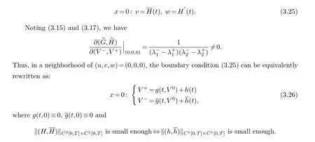
Moreover, it follows easily from the conditions ofC2compatibility for the original system that the mixed initial-boundary value problem (2.7), (3.20) and (3.25) satisfies the conditions ofC1compatibility at the point (t,x)=(0,0).By means of Lemma 3.1 that the theory on the semi-globalC1solution to the first-order quasilinear hyperbolic system, we can obtain the existence and uniqueness of the semi-globalC2solution to the original mixed initial-boundary value problem (1.1), (3.1) and (3.8) for case (2).We complete the proof of Theorem 3.2.

Proposition 3.2.Suppose that(2.3)-(2.4), (2.16)and(3.4)hold,considering the boundary condition:

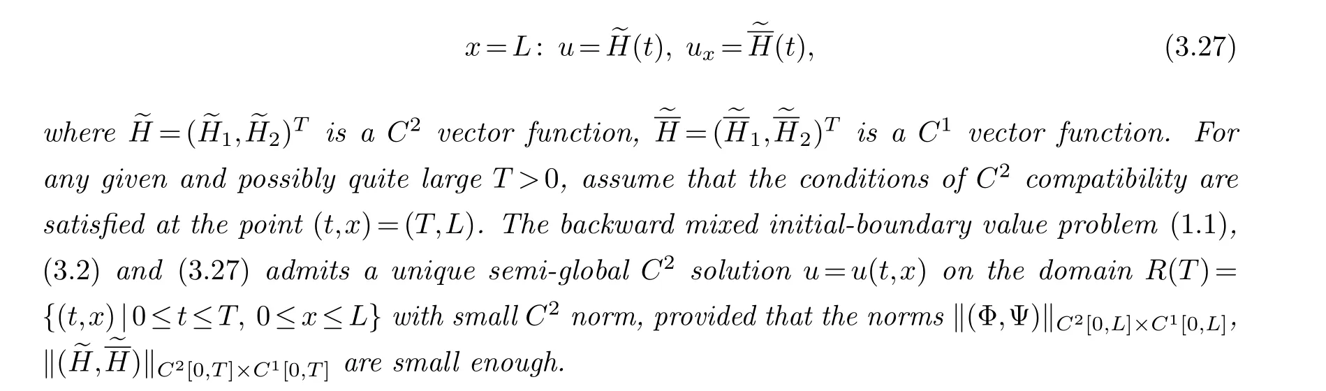
For case (3), the existence and uniqueness theory on the semi-globalC2solution to corresponding mixed initial-boundary value problem can be similarly obtained.

Remark 3.2.In the cases(1)-(3),we can also consider other boundary conditions that are satisfied the well-posedness of semi-global C2solution.

§4.Local exact boundary controllability

First, for case (1) we consider the corresponding local exact boundary controllability.

Theorem 4.1.(Local two-sided exact boundary controllability for case (1)):Suppose that αi,βi,ci(i=1,2),a,b are all C1functions with respect to their arguments.Suppose furthermore that(2.3), (2.16)and(3.3)hold.

In order to prove Theorem 4.1, it suffices to establish the following lemma.

Lemma 4.1.Under the assumptions of Theorem 4.1,if T>0is defined by(4.1),for any given initial data(?(x),ψ(x))and final data(Φ(x),Ψ(x)),where ‖(?,ψ)‖C2[0,L]×C1[0,L],‖(Φ,Ψ)‖C2[0,L]×C1[0,L]are small enough,system(1.1)admits a unique C2solution u=u(t,x)with small C2norm on the domain R(T)={(t,x)|0≤t≤T, 0≤x≤L},which satisfies simultaneously the initial condition(3.1)and the final condition(3.2).

Proof.Noting (4.1), there existsε>0 such that

Step 1 We first consider the forward mixed initial-boundary value problem for system(1.1) with initial condition (3.1), and the following artificial boundary conditions given on the endsx=0 andx=L:

wheref,gare any given vector function with smallC2[0,T1] norms, and satisfy the conditions ofC2compatibility at the points (t,x)=(0,0) and (0,L), respectively.By Theorem 3.1, this forward mixed initial-boundary value problem exists a uniqueC2solutionuf(t,x) with smallC2norm on the domainRf={(t,x)|0≤t≤T1, 0≤x≤L}.Especially, we have

Step 2 Next, we consider the backward mixed initial-boundary value problem for system(1.1) with final condition (3.2), and the following artificial boundary conditions given on the endsx=0 andx=L:

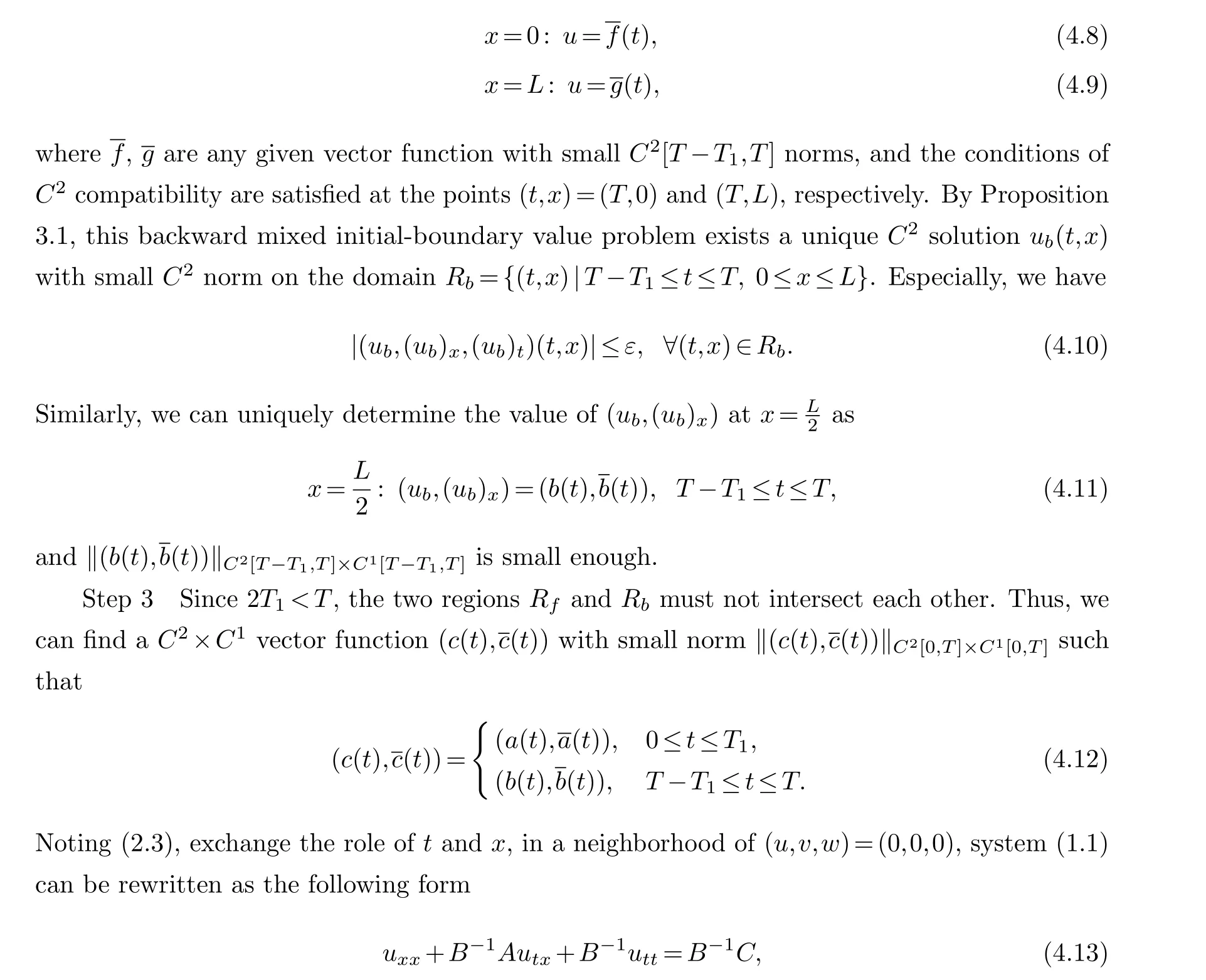
it is easy to see thatB-1AandB-1are still lower triangular.By (2.5)-(2.6), the second-order quasilinear system (4.13) can also be reduced to the following first-order quasilinear hyperbolic system:

Similarly, we can calculate that system (4.14) has 6 eigenvalues

Suppose that

which implies

Therefore,the first-order quasilinear system(4.14)is hyperbolic,in other words,the second-order quasilinear system (4.13) is hyperbolic.

Next, we consider the leftward mixed initial-boundary value problem for system (4.13) with final condition

Step 4 Similarly, we consider the rightward mixed initial-boundary value problem for system (4.13) with final condition (4.18) and boundary condition

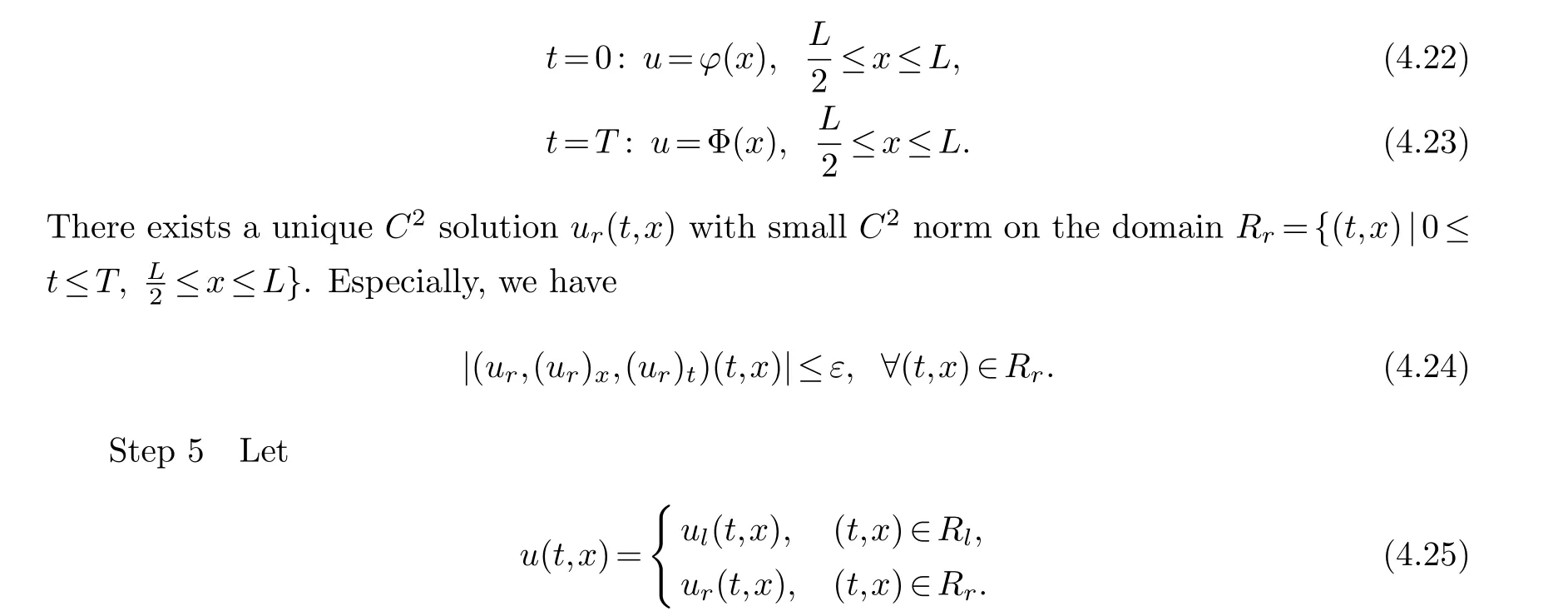
Thusu∈C2[R(T)], and it satisfies system (1.1) on the domainR(T).

The only thing left is to prove thatu=u(t,x) satisfies simultaneously the initial condition(3.1) and the final condition (3.2).

In fact, theC2solutionuf(t,x) andul(t,x) (resp.ur(t,x)) satisfy simultaneously the one-sided mixed initial-boundary value problem for system (1.1) (resp.(4.13)) with the initial condition

and the boundary condition (4.19) (resp.(4.22)).By the choice ofT1in (4.3), obviously, the maximum determinate domain of this one-sided mixed problem contains the triangular domain

The proof of Theorem 4.2 is established by the following lemma.

Lemma 4.2.Under the assumptions of Theorem 4.2,if T>0defined by(4.28),for any given initial data(?(x),ψ(x))and final data(Φ(x),Ψ(x)),where ‖(?,ψ)‖C2[0,L]×C1[0,L],‖(Φ,Ψ)‖C2[0,L]×C1[0,L]are small enough,for any given boundary function H(t)with small norm‖H‖C2[0,T]so that the conditions of C2compatibility are satisfied at the points(t,x)=(0,0)and(T,0),system(1.1)admits a unique C2solution u=u(t,x)with small C2norm on the domain R(T)={(t,x)|0≤t≤T, 0≤x≤L},which satisfies simultaneously the initial condition(3.1)and the final condition(3.2)and the boundary condition(3.6).

Proof.Noting (4.28), there existsε>0 such that

Let

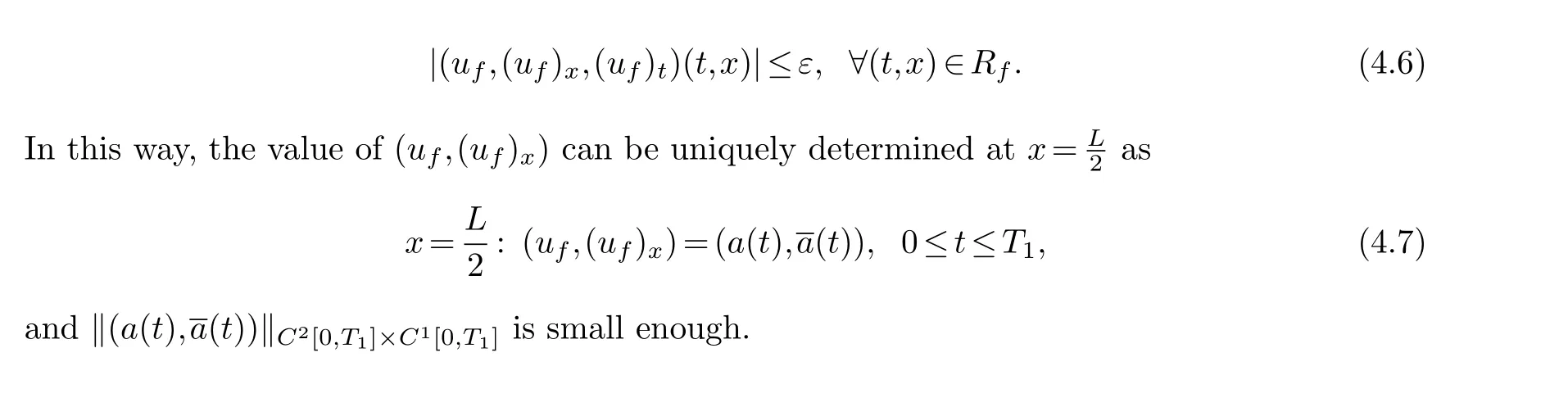
Step 1 First, we consider the forward mixed initial-boundary value problem for system(1.1) with initial condition (3.1), the boundary condition (3.6) on the endx=0 and any given artificial boundary condition(4.5)on the endx=L(in whichg(t)satisfies the same assumption).By Theorem 3.1, obviously, there exists a uniqueC2solutionuf(t,x) with smallC2norm on the domainRa={(t,x)|0≤t≤Tf, 0≤x≤L}and (4.6) holds.Thus, the value of (uf,(uf)x)can be uniquely determined on the endx=0 as

and the boundary condition

By Theorem 3.1, this rightward mixed initial-boundary value problem admits a uniqueC2solutionu=u(t,x) with smallC2norm on the domainR(T)={(t,x)|0≤t≤T, 0≤x≤L}.Especially, we have

Step 4 Similarly, theC2solutionu(t,x) anduf(t,x) satisfy simultaneously the one-sided mixed initial-boundary value problem for system(1.1)(resp.(4.13))with the boundary condition(4.35) and the following initial condition:

According to the choice ofTf(see (4.30)), the maximum determinate domain of this one-sided mixed problem contains the triangular domain

Thus, by the uniqueness ofC2solution to the one-sided mixed initial-boundary value problem(see [4] and [8]),u(t,x)≡uf(t,x) holds on the above domain and, in particular,u(t,x) satisfies(3.1).We can prove thatu(t,x) satisfies (3.2) in the same way.Thus,u(t,x) fits all the requirements of Lemma 4.2.

Now, we show the exact boundary controllability for other cases.For case (2), we only need to discuss the corresponding local one-sided exact boundary controllability on the endx=0, the following theorem can be obtained similarly.

Theorem 4.3.(Local one-sided exact boundary controllability for case (2)):Suppose that αi,βi,ci(i=1,2),a,b are all C1functions with respect to their arguments.Suppose furthermore that(2.3)-(2.4), (2.16)and(3.4)hold.Let

Similarly, for case (3), we only need to consider the local one-sided exact boundary controllability on the endx=L.We omit the details.

Remark 4.1.The single second-order quasilinear hyperbolic equation utt+a(u,ux,ut)utx+b(u,ux,ut)uxx=c(u,ux,ut)studied in[17]can be regarded as a special case of system(1.1)when n=1in this paper.