
Calculation of Available Transfer Capability Using Hybrid Chaotic Selfish Herd Optimizer and 24 Hours RES-thermal Scheduling
2024-01-16 07:46,
,
(1.Department of Electrical Engineering,Dr.B C Roy Engineering College,Durgapur 713206,India;2.Department of Electrical Engineering,Kalyani Government Engineering College,Kalyani 741235,India;3.Department of Electrical Engineering,NIT Durgapur,Durgapur 713209,India)
Abstract: As fossil fuel stocks are being depleted,alternative sources of energy must be explored.Consequently,traditional thermal power plants must coexist with renewable resources,such as wind,solar,and hydro units,and all-day planning and operation techniques are necessary to safeguard nature while meeting the current demand.The fundamental components of contemporary power systems are the simultaneous decrease in generation costs and increase in the available transfer capacity (ATC) of current systems.Thermal units are linked to sources of renewable energy such as hydro,wind,and solar power,and are set up to run for 24 h.By contrast,new research reports that various chaotic maps are merged with various existing optimization methodologies to obtain better results than those without the inclusion of chaos.Chaos seems to increase the performance and convergence properties of existing optimization approaches.In this study,selfish animal tendencies,mathematically represented as selfish herd optimizers,were hybridized with chaotic phenomena and used to improve ATC and/or reduce generation costs,creating a multi-objective optimization problem.To evaluate the performance of the proposed hybridized optimization technique,an optimal power flow-based ATC was enforced under various hydro-thermal-solar-wind conditions,that is,the renewable energy source-thermal scheduling concept,on IEEE 9-bus,IEEE 39-bus,and Indian Northern Region Power Grid 246-bus test systems.The findings show that the proposed technique outperforms existing well-established optimization strategies.
Keywords: Available transfer capability (ATC),biogeography-based optimization (BBO),chaotic map,chaotic selfish herd optimizer (CSHO),grey wolf optimizer (GWO),optimum power flow (OPF),power generation cost (PGC),renewable energy sources (RES),selfish herd optimizer (SHO)
1 Introduction1
According to the North American Electric Reliability Council (NERC),the definition of “available transfer capability” (ATC) is the amount of additional power that can be moved over the lines that are already in place without infringing on the power systems’ limits.The hourly and daily ATC data must be openly accessible as per the guidelines of the Federal Energy Regulatory Commission (FERC).Presently,the complexity of power systems is very high because the modern frameworks and distributed generators (DGs)are connected to the grid.
The system operator must provide ATC in an open-access,publicly assessable domain on an hourly and daily basis[1].According to the World Bank and Central Electricity Authority (CEA) India[2-3],the world’s power demand is increasing rapidly.Constructing a new transmission line for highly populated countries such as India and China is almost impossible.An ATC assessment provides appropriate information to ensure that these types of power transactions continue to take place over the current transmission lines without infringing on the limits of the power system[1,4-5].
Therefore,the real-time calculation of ATC always adds an extra burden to the optimization process.The benefit of real-time ATC assessment is that assessment occurs during the actual operation of power networks when power transactions are happening.An operator can have ten times more power transaction conditions in the existing network if the ATC is known in advance.Scheduling renewable energy sources (RESs) with thermal generation units introduces additional uncertainties that require careful consideration.This problem cannot be ignored from a financial engineering perspective[1].In the present era,power system networks involve grids,DGs,RESs,and flexible AC transmission systems (FACTS),which make power-flow equations much more complex and nonlinear[6].Hence,known linearization methods cannot accurately evaluate the ATC.Several computational techniques have been used to obtain an accurate ATC by maintaining the voltage stability,thermal limit,reactive power generation limit,and other power system constraints within limits;the techniques are listed below.
(1) Using an optimal power flow (OPF) method[7].
(2) Using a distributed contingency analysis method[8].
(3) Using a conceding voltage stability monitoring process[9-10].
(4) Using a distributed state estimations process[11-12].
(5) Using a distributed control for distribution power networks[13-14].
Some standard optimization techniques,such as biogeography-based optimization (BBO),grey wolf optimization (GWO),and selfish herd optimizer(SHO),are widely used to evaluate the OPF.Hence,these optimization tools can also be used for ATC calculations.Therefore,a real-time ATC can be determined by modeling a multiarea OPF problem that considers both the equality and inequality criteria.Time and memory complexities are no longer major issues for modern computers.Meta-heuristic algorithms are a class of computational techniques employed to obtain near-optimal solutions to optimization problems.Genetic algorithms are well suited for addressing combinatorial optimization problems because of their ability to efficiently identify a solution of satisfactory quality within a reasonable time frame.Meta-heuristic algorithms are a potent set of procedures that aim to optimize one or more objective functions for a particular problem while considering the constraints and limitations.The techniques in question are problem agnostic,meaning that they do not rely on any particular characteristics of the problem at hand and are thus applicable to a broad spectrum of problems.Metaheuristic algorithms possess numerous advantages over nonmetaheuristic techniques.These advantages include the capacity to discover approximate solutions to optimization problems,wide-ranging applicability,and the ability to generate nearly optimal solutions in a computationally efficient manner.Furthermore,the computation of ATC using the OPF method involves intricate nonconvex and nonlinear methodologies.Therefore,the classical techniques are considered inadequate.Hence,the use of metaheuristics is required.Therefore,the ATC can be evaluated in real time using OPF by applying metaheuristic techniques.Briefly,the main arguments of this study are as follows.
(1) SHO and chaotic selfish herd optimizer(CSHO) algorithms are employed to formulate the multiarea ATC problem using OPF.
(2) Usually the generation cost is not considered when computing the ATC.However,in this study,a multi-objective optimization problem that includes generation costs is considered[15-17].
(3) According to the ATC calculation,the integration of hydro-wind-solar units with thermal power plants aims to reduce the expenses incurred in the production of active power and safeguard the environment.
(4) The problem formulation presented in this article considers the scheduling of thermal,hydro,wind,and solar energy systems,along with the fluctuation in energy demand over a 24-h period and enhancement of the ATC during this time frame[18-21].
The remainder of this paper is organized as follows.Section 2 presents a clear mathematical representation of the proposed problem,including relevant information on wind,solar,thermal,and hydroelectric resources.In Section 3,we describe the implementation of the proposed hybrid chaotic selfish herd optimizer and selfish herd optimizer algorithms in detail.Section 4 presents the investigation on the use of the aforementioned method under different test conditions,namely the IEEE 9-bus,IEEE 39-bus,and Indian Northern Regional Power Grid (NRPG)246-bus systems.Finally,we conclude the paper and discuss future implications in Section 5.
2 System modelling using mathematics
The mathematical foundations for wind,solar,hydrothermal,and ATC calculations are applied individually in this section.
2.1 Generation of wind energy and its cost
The generation of wind power is unpredictable[22-24].The probability density function in Eq.(1) can be used to forecast wind speed,as shown below[25]
The cumulative density function (CDF) for wind speed is denoted by Eq.(2)
A linear model can be used to illustrate the relationship between wind speed and viability of wind power generation,as shown in Eq.(3)
The authors computed the likelihood of wind power under wind and zero wind conditions using Eqs.(4)and (5) as follows
wherecdwis a random variable (wnd) obtained using Eqs.(4) and (5) that can be rewritten as follows
Wind power output is not constant because of variations in wind speed.Consequently,the amount of wind power produced is sometimes less than the demand (an overstated scenario),whereas at other times,it is greater than the load demand (under the estimated scenario).Both scenarios include two additional cost factors for the production of wind power: overestimation and underestimation costs.The formulas for underestimating and overestimating costs can be stated as follows
The “direct cost of wind power” or the money spent buying electricity from a wind farm operator in response to a specific demand,is expressed as follows
Thus,the following are the wind power production estimates for each period,which considers the potential for under and overestimation,as well as the direct cost of wind generation
whereNwndis the total number of wind generators.
2.2 Solar energy and its cost of production
In a solar power plant,the amount of energy produced is proportional to the amount of incoming solar radiation (SIs) and the surrounding temperature (Tamb).Consequently,the solar energy output may be written as
The total solar share (Stot) from the units that have been placed may be regulated by whether or not the solar panels are turned ON or OFF.
The solar share,denoted byStot,has a maximum limit that is capped atxsolar% of the total demand power at any sub-intervaltwithin the total intervalT,and the method for determining that limit can be expressed in mathematical terms as follows
To obtain the greatest advantage from the installed solar capacity,clients are assessed a penalty factor.Therefore,the cost of the difference between the installed power capacity and amount of solar power produced is as follows
2.3 The economics of producing electricity from hydropower
Compared with other forms of power generation,the costs associated with operating a hydropower plant are minimal[26-27].Combining a hydropower-producing unit with a thermal power plant is a viable option to reduce fuel and pollution costs[28].Production of hydroelectric power,denoted byPHYi,t,may be expressed in terms of water flow rate and reservoir capacity as follows
where HO1,i,HO2,i,HO3,i,HO4,i,HO5,iand HO6,iare the coefficients for hydroelectric power generating units,and Voli,tand disqi,trepresent the water volume of theith unit and discharge rate water ofith unit,respectively[29].
2.4 Generation of thermal electricity and its associated costs
The valve-point effect and quadratic function are often used to illustrate how a thermal power generator operates,as follows[30-31]
where the total number of thermal units is given byNgenTH;αi,βi,andγiare the fuel coefficients;e1iande2iare the valve point loading effect constants;andPthminiis the lowest active power production of theith thermal unit.Thus,the active power production cost for the thermal unit,along with the solar,wind,and hydro units,may be calculated as follows
where the scalar constantwγmaps water volume discharge to the price of generating an equal amount of electricity[32-34].
2.5 Formulation of the ATC and RES-thermal scheduling issue
In this study,the OPF concept is used to address the challenges faced by ATC.A target function or cost function is created to maximize electricity transmission from a source region of generating units to a sink region of loads through a network of transmission or tie lines without breaching the limits and restrictions imposed by the operation of the power grid.The thermal limit of a power line is the maximum power that can be transmitted across it.The purpose is to develop a mathematical formulation of the ATC cost function.Unlike most cases in which only the cost of producing power is considered,both the ATC and power generation cost (PGC) are considered here.This study focused on three major situations.
(1) Case A: Schedule RES with thermal units strategically to minimize the cost of active power production[35-37].
(2) Case B: Maximize ATC without exceeding restraints imposed by the electrical system.
(3) Case C: Maximize ATC while minimizing the cost of producing electricity from RES (multiobjective).
Therefore,the cost function may be expressed as
For the objective function,TLφ,Vφ,φTLA,andφgenare positive scalar values.Using these scalar factors,a single or multi-objection cost function may be produced with appropriate weighting.Power flow through certain lines can be increased to improve ATC,as indicated below
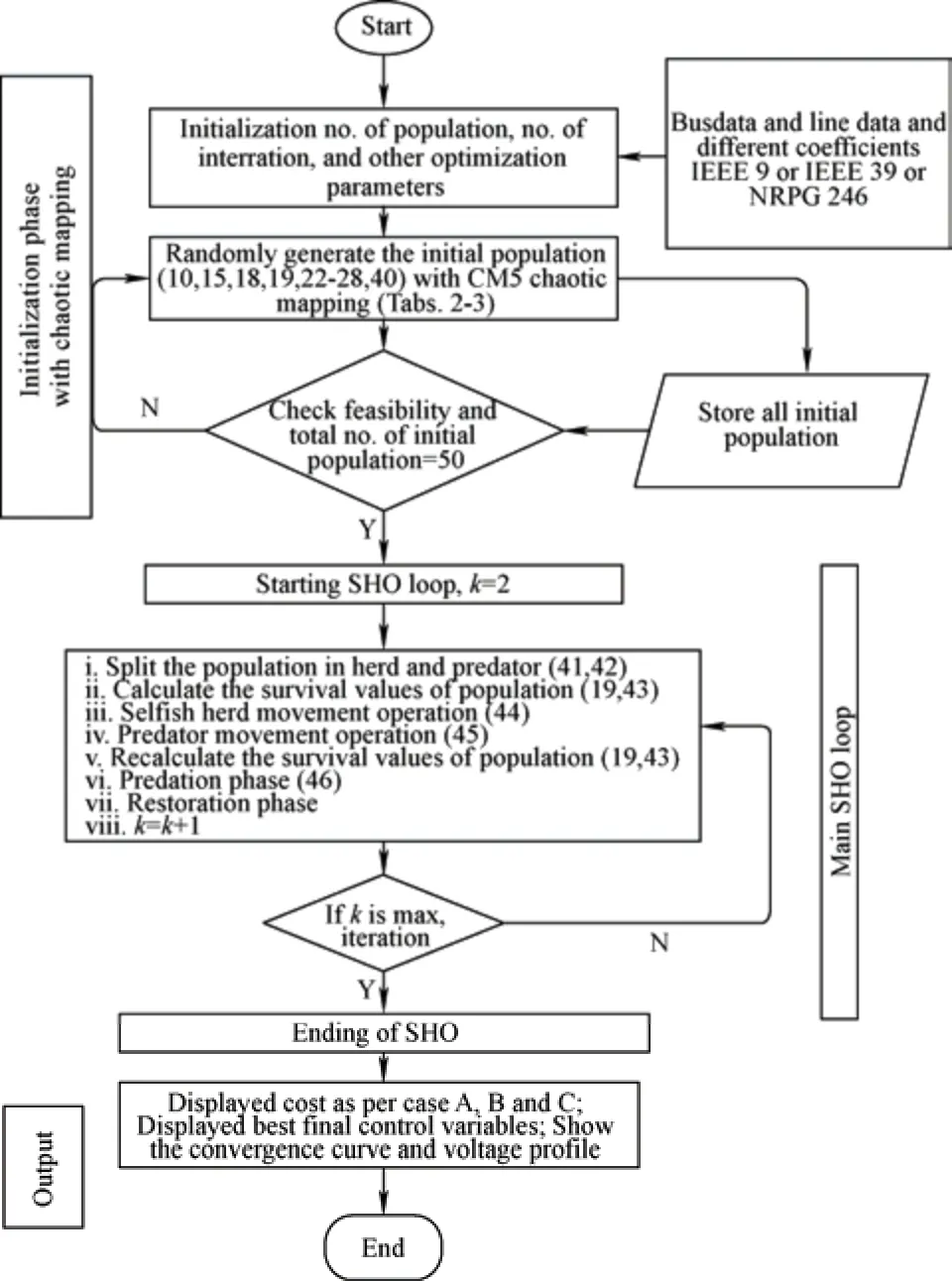
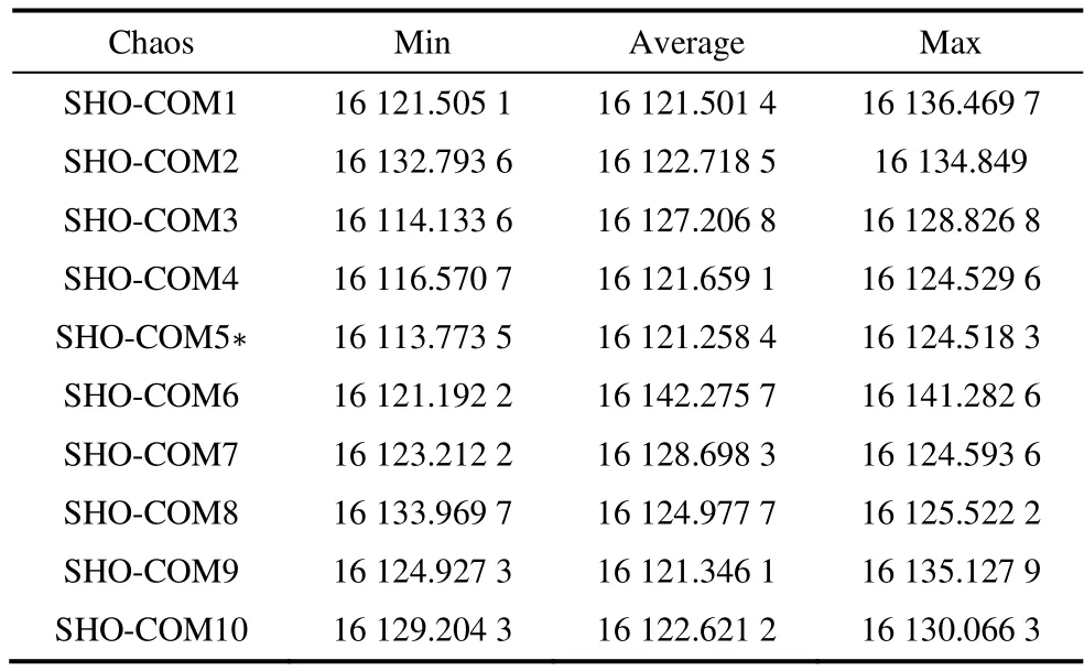
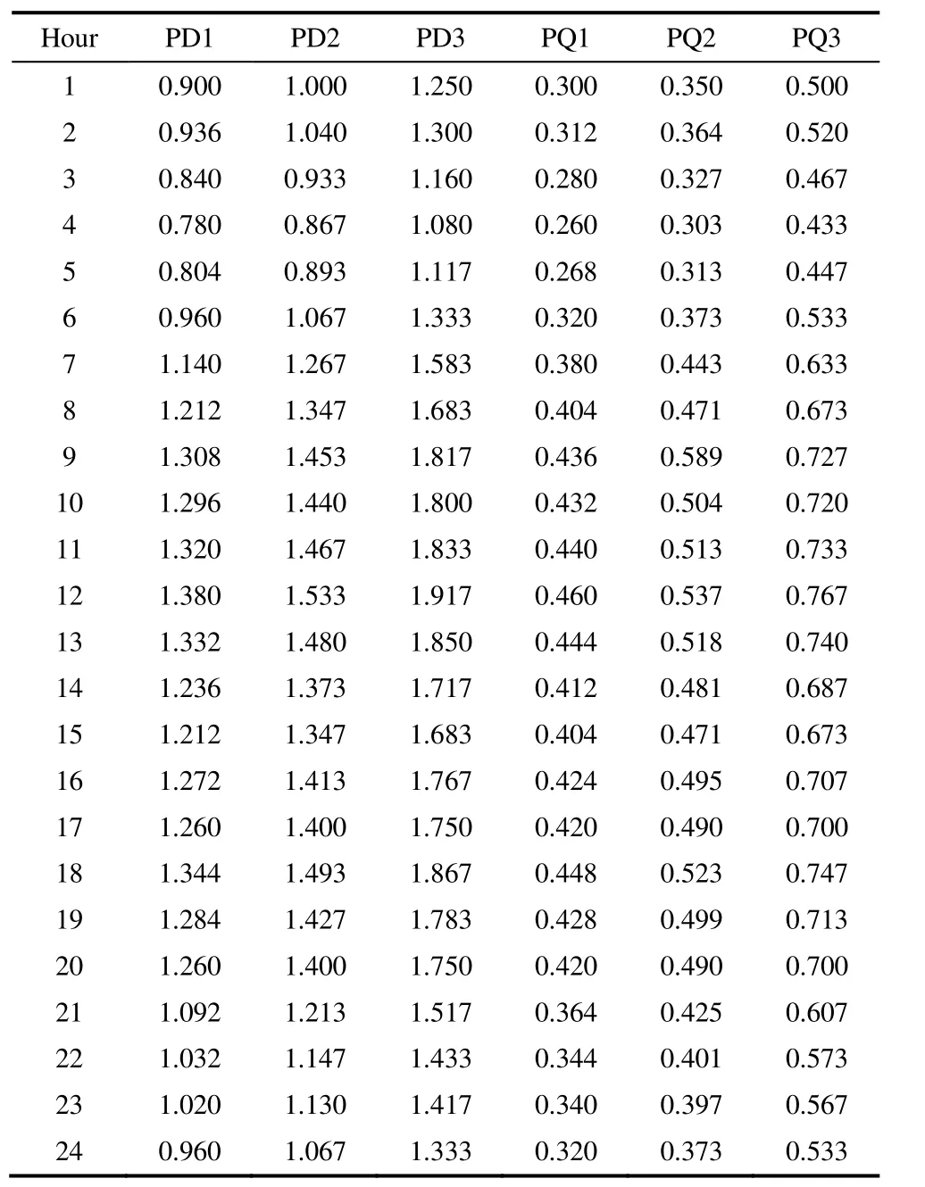
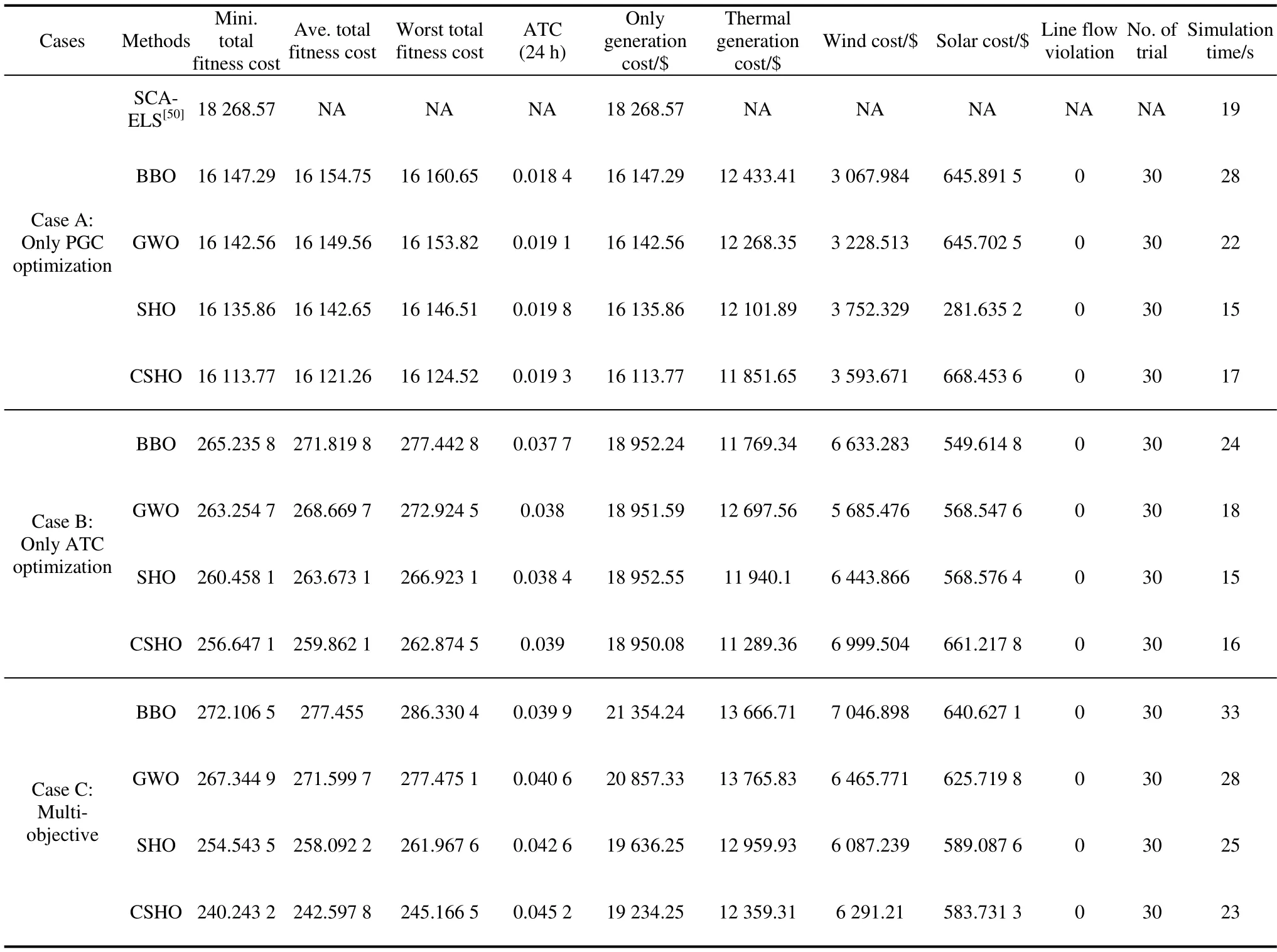
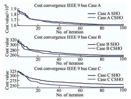
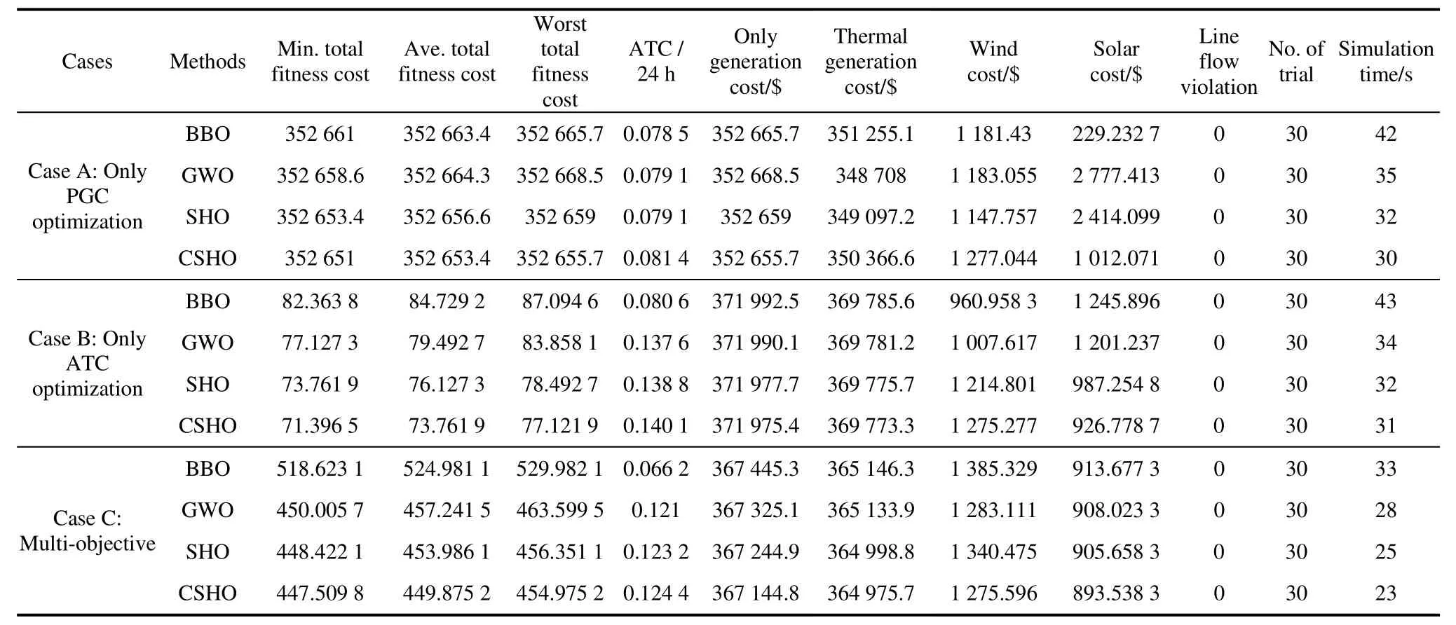
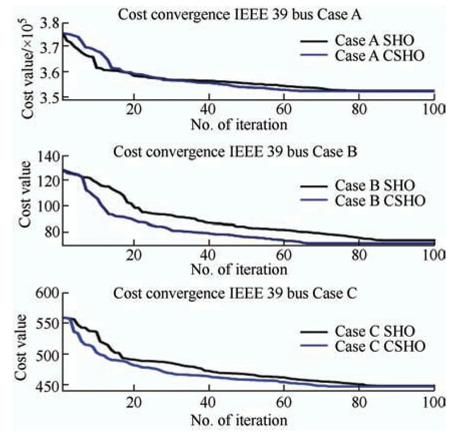
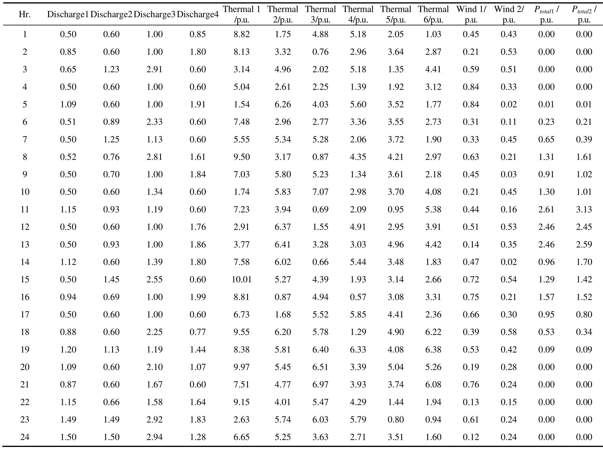
whereSTLiis the power flowing down the ith line andSTLiBis the base power flowing along the line.A mathematical safeguard against transmission line overload has been included into the cost function in the form of the following if statementSTLmaxi The following is the equality requirement placed on load flow The following are the limits placed on the production of voltage,active power,and reactive power whereNBUSandNGENare the total bus and generator bus counts,respectively.,,andare the maximum and lowest voltages and active and reactive power production limitations,respectively,in the IEEE test system.The test system’s tap setting transformer and shunt reactor compensations are as follows whereNSHandNTare the total number of shunt reactors and tap-transformers,respectively.Their minimum and maximum values are denoted by the superscripts min and max,respectively.The values of the scalar constants used in Eq.(19) are provided in Tab.1,in which the scalar factor varies depending on the specifics of the case. Tab.1 System parameters This section discusses several metaheuristic algorithms developed to address these issues,such as the proposed CSHO. Biogeography studies the emergence of novel species,movement of populations from one ecosystem to another,and extinction of populations elsewhere.In BBO,a habitat is conceptualized as an island (region)separated from other islands by physical distance.To qualify as an ideal residential location,a habitat must have a high habitat suitability index (HSI).Suitability index variables (SIVs) are used to describe the factors that make space habitable[38].The SIV index is assumed to be the habitat’s independent variable,and thus the HSI is dependent on it.The basic BBO method for solving optimization problems comprises two steps migration and mutation[39]. 3.1.1 Phase of migration During the migration phase of BBO,characteristics migrate to other islands and emigration from the population occurs,resulting in creation of the next set of solutions.Rates of emigration and immigration from and to thekth island may be modelled as shown in Eqs.(28) and (29) wherekλandkμare the immigration and emigration rates for thekth individual,respectively;Emax,Imax,andSmax,represent for thekth individual’s species count and the maximum number of species that may exist,respectively. 3.1.2 Phase of mutations The BBO mutation process is meant to increase the population density to sustainably feed on excellent solutions.At this stage,the mutation rate determines the random change in the habitat SIV index[40] Each of these potential habitats,or candidate solutions,is denoted bymSIVs (a vector),with each SIV consisting of the value of the associated control parameter andPkas shown in Eq.(31) In 2014,Mirjalili et al.[41-45]pioneered the implementation of the GWO.The algorithm addresses the mechanics of hunting and the democratic behavior of grey wolves living together in a pack in the wild.Grey wolves adhere to a very hierarchical and domineering social structure when they are in a pack.The order of the social dominance hierarchy is as follows. (1) Alpha wolves (α) (a female and a male): the pack’s highest-ranking leaders who make the decisions. (2) Beta wolves (β): subordinate wolves who assist the alpha. (3) Delta wolves (δ): responsible for relaying information to the higher two tiers. (4) Omega wolves: the lowest level in the wolf hierarchy that comprises infant and weak wolves who relay information to all other ranks. This social order,which comprises tracking,surrounding,and attacking prey,can be mathematically modelled as discussed in the following section. 3.2.1 Rank in society The optimal solution is designated as an alpha wolf(alpha),the second-best as a beta wolf (beta),and the third-best as a delta wolf (delta).The remaining candidate solution sets are assumed to be omega(omega).Although this described method,which is similar to a hunting mechanism,is mostly controlled by alpha,beta and delta also have an effect. 3.2.2 Phase of encircling prey The surroundings of the prey that successfully use the hunting mechanism may be mathematically defined as follows wheret0is the current iteration;XpandXware the position vectors for a prey and a grey wolf,respectively;CandAare coefficient vectors;rand1andrand2are two different random vectors in between[0,1];andais linearly reduced from 2 to 0 over the progress of said iterations.The three best solutions(Xpα,Xpβ,andXpδ) are saved including the latest positions of the omegas according to the current best position.The final position,Xw(t0+2) is defined by the positions of alpha,beta,and delta in the search space. whereiisα.SimilarlyX2andX3can be evaluated by replacingiasβandδ,respectively. During the course of the simulation,the alpha,beta,and delta wolves each make an educated guess on the location of the prey.IfA>1,then the candidate solutions have moved away from the prey,and ifA<1,then the candidate solutions have moved closer to the prey. The SHO method is concerned with how a prey animal(within a herd) might improve its chances of surviving a predator assault;however,it does not consider how this would affect the chances of surviving prey animals[46]. 3.3.1 Phase of initializing the population The first phase of the SHO algorithm involves random construction of predators and prey.During initialization,the total size of theAofNpopulation is set toA=a1,a2,…,ai,…,aN,whereaiis the position of an individual.Eachn-dimensional search space solution isai,j=[ai,1,ai,2,…,ai,n].The initial population is produced randomly as follows 3.3.2 Survival value assignment stage Notably,when predators and prey interact,each member of a pack or herd has a unique survival profile,and thus,a unique likelihood of surviving an attack or killing a target animal.The mathematical representation of this survival valueSiaVfor each individual animal inn-dimensional search space is as follows wherefbestandfworstare the best and worst fitness values recorded thus far depending on the pace of convergence. 3.3.3 A selfish herd’s structure There are a few distinct positions within a herd’s hierarchy.During aggregation,the herd leader controls the direction of the prey.Many members of a herd decide where to go based on their shared knowledge of how to stay alive and the proximity of other members of the herd.Those who abandon the herd choose their own path independent of the rest of the quarry. 3.3.4 Operators of herd movements The SHO method is regulated by two distinct evolutionary theories.One set of leaders in the herd functions as the operator of the herd’s movement,whereas another set of leaders in the herd acts as the operator of desertion and follows the movement.All animals in a selfish herd learn crucial details about one another during these operational movements,such as how far away they are from other members of the aggregation and the value of their own survival. 3.3.5 Operators of predator movement The danger of predation for solitary individuals is greater than that for herd members.Mass motion causes a predator to become disoriented and misjudge where to launch an assault.An SHO model predicts how a predator’s pack will travel in relation to a herd based on how well its members will be able to avoid being killed by the herd and how far away from it they are when the attack begins. 3.3.6 Probabilities of pursuing In SHO,the equation for the pursuit probability is 3.3.7 Period of predation In the SHO technique,the predation phase determines how the prey and predator interact.It is thought that after both the pack of predators and the selfish herd(prey) move,the exclusion of a solution from the current set of solutions and the dangerous area can be shown as follows forn-dimensional space 3.3.8 Period of restoration Predation causes the size of prey populations to change dynamically throughout the year.This effect is reflected in the manner in which the SHO algorithm returns the number of prey items.By replacing the members of the herd who were kicked out and letting them mate,the original balance of the herd’s population is restored. In this section,the authors describe their devised hybrid SHO algorithm,which uses the idea of a chaotic scale factor.In a chaotic system,the most important concerns are the preliminary factors and sensitivity of the conditions.The process of initializing the SHO algorithm has been significantly aided by the chaos concept.Therefore,to achieve better convergence,a hybridization of chaos and SHO is proposed in this study.According to previous papers[47-48],chaotic combinations are often nonlinear stimulation systems.Therefore,the response of chaotic combinations depends on both the changes in the system parameters and the starting expressions.Numerous chaotic map iterations have been proposed.In this article,ten distinct chaotic maps were considered.These maps are as follows: circle,cubic,logistic,Gaussian/mouse,iterative,sinusoidal,sine,singer,tent,and piece-wise[49].A quick tabulation of these maps is presented in Tab.2.After combining theabove ten chaotic maps with the SHO algorithms to create an initial SHO population for resetting the simulation,the optimal chaotic map was chosen for use in the IEEE 9-bus,IEEE 39-bus,and Northern Regional Power Grid (NRPG) 246-bus systems. Tab.2 Names of the different chaotic maps and their mathematical expressions In this section,the implementation of the proposed hybrid chaotic SHO is explored using the flowchart shown in Fig.1.In a previously described technique,the SHO-COM5 A chaotic map is interchangeable with several other possibilities.As presented in Tab.3,SHO-COM5 was used in this study. Fig.1 Flow chart of CSHO Tab.3 The chaotic map results for Case A using the 9-bus system In this study,three different test systems were used to assess the efficacy of the recommended algorithms:IEEE 9-bus,IEEE 39-bus[50-51],and NRPG 246-bus[52]systems.Each of these test systems had a different number of buses.Thirty trial runs were performed for each test case and each optimization,utilizing data from the MATPOWER toolkit and other sources[50-55].Fifty individuals were chosen randomly from the entire population to represent each incident.All test cases were implemented on a system made by ASUS with a Ryzen 5 processor running at a speed of 2 GHz,Windows 10 (Home,64 bits),12 GB of RAM (DDR3)memory,and Matlab 2020a.In this study,30 random trial runs were performed on a 9-bus system to generate ten different chaotic map variants for Case A.A comparative analysis is shown in Tab.3.Compared with other chaotic maps of hybridization,the iterative chaotic map,also known as COM5,provides the most desirable results when used in conjunction with SHO.Therefore,an iterative chaotic map hybridization with SHO was considered for all examples utilized in this study.A standard MVA of 100 was used for the calculations. In the 9-bus test system,there are nine buses and six generating units;two are hydro units,one is a wind unit,two are solar units (consisting of 13 panels each),and one is a thermal unit.The 9-bus test system was designed to simulate real-world conditions.The active and reactive loads are denoted as (PD1,PQ1),(PD2,PQ2),and (PD3,PQ3),respectively,and tabulated for a 24 h load,as shown in Tab.4.There were three load buses: buses 5,7,and 9.In this study,the ATC computation is performed using line number 2,which extends from bus 4 to bus 5.In the IEEE 9-bus test system,the control variables consisted of two discharges for two hydro units,active power generation from one thermal unit,active power generation from one wind unit,and active power generation from two solar generation units,six generating bus voltages,two taps that set the transformer tap positions,and two shunt compensation Vars.Consequently,the total number of control variables was 16.Subsequently,three instances were investigated in chronological order.The authors’primary goal in the first scenario,which they refer to as Case study A,was to reduce the cost of generation to the maximum possible extent.Tab.4 shows the active and reactive power demands round the clock for 9 bus.As shown in Tab.5,the reduction in total cost after 30 random trial runs using BBO was determined to be $16 147.286 5/24 h,which is superior to that achieved using a sine cosine algorithm (SCA) in conjunction with economic load scheduling,$18 268.570/24 h[50].Moreover,GWO yields better results for the same $16 142.562 3/24 h,whereas the proposed algorithm in conjunction with the COM5 method yields the best result of $16 113.773 5/24 h.Tab.6 shows the demand for 39 bus system.It is also noteworthy that in this case,the total thermal cost is reduced to $11 851.649 3/24 h,and the control parameters for these test studies,including water discharge,wind and thermal generation,six generating bus voltages,two tap-setting transformers,and two shunt capacitors injected with Var and two solar units(panel-wise states),for 24 h are provided in Tab.7. Tab.4 Demand in the PU of a 9-bus system that is active and reactive round the clock Tab.5 Maximization of savings by comparing costs over 24 h and 9-bus using various approaches Tab.6 PU demand of a 39-bus system that is active and reactive round the clock Tab.7 Parameters for maximizing CSHO’s cost-effectiveness in a 9-bus system sole generator (PGC) Observations indicate that thirteen solar panels in each solar unit have two states,ON and OFF,represented by “1” and “0”,respectively.Fig.2 depicts the costs ($/24 h) of the various described algorithms for all instances and Fig.3 shows a 3D picture of how the voltages of all nine buses changed over the course of 24 h.In scenario B (maximum ATC) for the suggested CSHO,the maximum values are 0.039 p.u.for 24 h,which is the best of the optimization strategies presented.Case study C concludes the discussion of multi-objective optimization by minimizing the total cost and maximizing the ATC.All controlled parameters are shown in Tab.8.Again,the CSHO approach delivered the best results of$240 243.2/24 h compared to other suggested algorithms based on 30 separate trial runs,with all control parameters shown in Tab.9.In Fig.3,the voltage profiles of all nine buses are shown in 3D for all times in a 24-h period.In addition,Tab.10 summarizes the lowest (best),average,and maximum(worst) production costs of other approaches for each case’s 30 unique trial runs.The simulation results demonstrated the computational efficacy of the proposed CSHO method. Fig.2 The cost-effectiveness of the 9-bus system in a range of simulations Fig.3 Voltage across a 9-bus system subjected to a variety of stress conditions (Bus voltage of IEEE 9 bus: 24 h) Tab.8 All parameters for ATC optimization by CSHO for 9-bus system Tab.9 For a 9-bus system,CSHO’s full set of multi-objective optimization parameters Tab.10 Maximization of savings by comparing prices over 24 h with 39-bus using various approaches The 39-bus test system has 14 generating units: four hydro units,two wind units,two solar units (each consisting of 13 panels),and six thermal units.There are 39 buses in the system.There are 25 load buses with a total active base load demand of 61.566 p.u.,total reactive base load demand of 13.429 p.u.,and load demand over a period of 24 h varied according to the H factor,as shown in Tab.4.Subsequently,three instances were investigated in chronological order.In the first case,the authors were only concerned with minimizing the cost of generation;in the second case,they were concerned with maximizing the ATC;and in the third case,they were concerned with minimizing the cost while also maximizing the ATC (a multi-objective problem).These three cases were designated as A,B,and C,respectively.Within the context of this study,the ATC calculation considers Line No.9,which extends from Bus 4 to Bus 14.In the first scenario,called “Case A” by the authors,they focused only on lowering the cost of making electricity.According to Tab 10,the minimal total cost that may be achieved with BBO after 30 random trial runs is$352 660.989 5/24 h.In comparison,SHO delivers$352 653.383 19/24 h,whereas the suggested CSHO with CM5 delivered $352 651.017 8/24 h.Fig.4 shows the convergence curves,which indicate how much better the suggested CSHO is than what is already being used.All produced bus voltage magnitudes are displayed in Fig.5.Tabs.11-13 show the control parameters under different case studies and the ON/OFF statuses of the solar units are listed in Tab.14.Tab.11 shows the discharges,thermal generation,and wind generation for the CSHO over the course of 24 h.Considering the suggested CSHO,the maximization of ATC produces the highest value of 0.140 1 p.u.for 24 h,which is the best among all optimization strategies covered in this study.The control parameters for the CSHO are listed in Tabs.12 and 13,respectively. Fig.4 Cost-effectiveness of a 39-bus system in a range of simulations Fig.5 Voltage across a 39-bus system subjected to a variety of stress conditions (Bus voltage of IEEE 39 bus: 24 h) Tab.11 Total cost minimization of discharge and active power production for CSHO in a 39-bus system (PGC only) Tab.12 Optimization of CSHO for 39-bus system using just discharge and active power generation (ATC only) Tab.13 The 39-bus system’s CSHO is multi-objective optimised for discharge and active power production Tab.14 Status of CSHO Case A,B,and C solar panels’ ON/OFF switches in the IEEE 39-bus system Finally,the authors discussed multi-objective optimization by focusing on lowering the total cost while increasing the ATC,as shown in Case C.Compared to the other algorithms,the CSHO approach yielded the best results,with a value of $447.509/24 h.This was performed while considering 30 separate trial runs,and the values for all control parameters are shown in Tabs.11-13 for respective best run.Fig.5 shows a three-dimensional picture of how the voltage changes over 24 h in each of the three scenarios. In addition,research is being conducted on the NRPG 246-bus test system.All information was gathered from published research[52,55].According to previous reports,bus 40 was used as the source,bus 200 was used as the sink,and the ATC discovered in Ref.[52]is 3.228 2 p.u..BBO,GWO,and SHO were compared to determine the effectiveness of the CSHO.As indicated in Tab.15,applying CSHO results in an ATC of 3.291 6 p.u.,which is significantly better than the results obtained by BBO (3.255 2 p.u.),GWO(3.276 5 p.u.),and SHO (3.280 8 p.u.) without violating any power system constraints.This is the case even though none of the other methods caused violations. In this study,we discuss a new strategy for ATC computation and power cost optimization that uses hydro,solar,and wind power.The proposed method,called the CSHO method,has been investigated and shown to be more efficient than previous metaheuristic optimizations in terms of the number of iterations and cost values.It also exhibits better convergence properties.It is necessary to consider both the unpredictability of wind power and load requirements.Another purpose of this study is to include solar,wind,and hydro units in typical thermal-producing units to decrease the total cost of active power production.The following is an outline of the outcomes produced by the proposed methodology.Similar heuristic approaches,such as SCA,BBO,GWO,and SHO,all produced similar results,which were shown in the most recent study.Utilizing the IEEE 9-bus is one way to demonstrate the effectiveness of the proposed solution.Test systems for the IEEE 39-bus and NRPG 246-bus,including three separate use cases were examined.In every case,both the convergence characteristics and efficiency of computing of the new method are much better than those of the old methods.This article discusses the difficulties of ATC and RES-thermal scheduling for 24 h,which adds to the overall uniqueness of the study.
3 Implementing the proposed algorithms
3.1 Incorporating the BBO algorithm
3.2 Incorporating the GWO algorithm
3.3 Incorporating the SHO algorithm
3.4 An introduction of chaotic maps

3.5 Issues with CSHO implementation
4 Case studies and observations
4.1 Research and findings of the 9-bus test system


4.2 Research and findings of the 39-bus test system


4.3 Research and findings of NRPG 246-bus test system
5 Conclusions
 Chinese Journal of Electrical Engineering2023年4期
- Chinese Journal of Electrical Engineering的其它文章
- A Review of Isolated Bidirectional DC-DC Converters for Data Centers*
- Review of Hybrid Packaging Methods for Power Modules*
- Vibration Reduction and Torque Improvement of Integral-slot SPM Machines Using PM Harmonic Injection*
- Filtered High Gain Observer for an Electric Vehicle’s Electro-hydraulic Brake: Design and Optimization Using Multivariable Newton-based Extremum Seeking
- Improved Approaches Toward Analysis of Electromagnetic Processes in Electrodynamical Devices Based on the Theory of Electromagnetic Field
- A Novel Modified Fuzzy-predictive Control of Permanent Magnet Synchronous Generator Based Wind Energy Conversion System