Dynamical Analysis of a Toxic-phytoplankton-zooplankton Model with Chemotaxis and Allee Effects

Dong Yuqin Chen Shaoyu Dai Binxiang

(1.School of Mathematics and Statistics,Central South University,Changsha 410083,China?2.Public Course Department,Enshi Polytechnic,Enshi 445000,China)

Abstract This paper demonstrates the global existence and boundedness of the solutions of a toxicphytoplankton-zooplankton model with chemotaxis and Allee effects in a smooth bounded domian with no-flux boundary condition.This result holds for arbitrary spatial dimension and small chemotaxis coefficients.It is also proved that the positive homogeneous steady state loses its stability when the chemotactic coefficient surpasses a threshold value,and the nonhomogeneous steady states bifurcate from the homogeneous steady state.Finally a numerical simulation is performed.

Key words Chemotaxis Toxic phytoplankton Zooplankton Allee effect

1 Introduction

Plankton refers to drifting organisms that live in waters such as oceans,lakes and rivers,and are divided into phytoplankton and zooplankton.Phytoplankton are important producers in marine ecosystems and are the basic link of the food chain? zooplankton control the number of phytoplankton through predation,and at the same time,as a bait for high-level nutrients such as fish,its quantitative changes can directly affect the amount of resources of fish and other species,and play an important role in the structure and function of marine ecosystems[1,2,3].However,in most aquatic ecosystems,there is a species of phytoplankton that can release toxin substances,and toxin-producing phytoplankton(TPP)release toxic substances in water to reduce zooplankton growth by decreasing grazing pressure[1].Chattopadhyay et al.[4]showed through field studies that when a specific harmful phytoplankton erupts,the cumulative effect of all the toxins released may affect other organisms,leading to mass deaths.There are many phytoplankton that can produce toxins such as:the motile stage of Alexandrium,the benthic Gambierdiscus and so on.

Chattopadhyay et al.[4]considered the following nonlinearly coupled ordinary differential equations through field sampling and observation

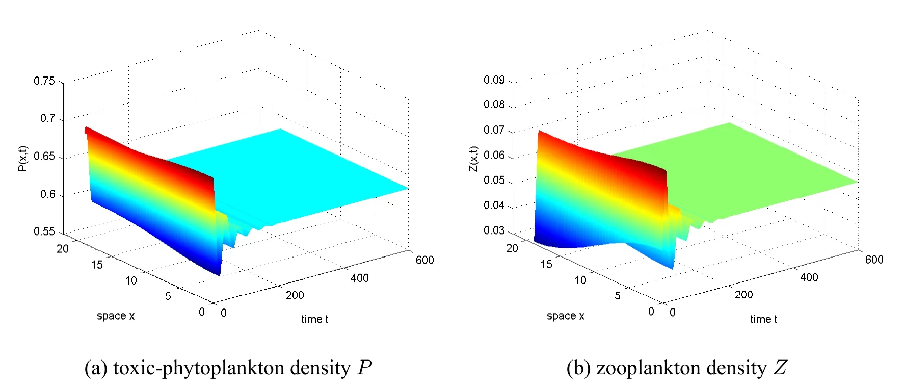
wherePis the population density of TPP andZis the population density of zooplankton?the population of TPP satisfies the logistic growth pattern?f(P) represents the functional response for the grazing of phytoplankton by zooplankton andg(P) represents the distribution of toxic substance which ultimately contributes to the death of zooplankton populations?r,K,α,β,μ,andθare all positive constants which respectively represent:the intrinsic growth rate of the TPP population,the environmental carrying capacity of the TPP population,the predation rate of zooplankton to the TPP population,the proportion of biomass consumed by zooplankton growth,the mortality rate of zooplankton,and the toxin release rate of TPP population.They showed that when the predator reaction functionf(P)is Holing-I,and the distribution functiong(P) of toxic substances is Holling-II,the positive equilibrium point of the system is globally asymptotically stable.And in the same year,they also proved that for a corresponding model with discrete time delay,the positive equilibrium point of the system is locally asymptotically stable at 0 <τ

In 1931,Warder Clyde Allee proposed that intraspecific cooperation could lead to inverse density dependence,and expanded this view in his famous book Animal Ecology,published in 1949.The Allee effect describes a situation in which smaller populations are affected by a positive correlation between population growth rate and density,which increases the likelihood of their extinction[5,6,7].The most common consequence of the Allee effect is the generation of a critical density threshold [8].The Allee effect is generally divided into two main types:the weak Allee effect(or non-critical Allee effect)and the strong Allee effect(or critical Allee effect),where the weak Allee effect has a lower per capita growth rate at low population densities but has never experienced a negative per capita growth rate and therefore does not exceed the critical threshold [8].The strong Allee effect refers to that when the population size falls below a critical threshold,the population growth rate is negative and the average population declines,and when the population size stays above this threshold,the per capita growth rate is positive and the average population growth rate finally converges to the carrying capacity[6,8,9,10].The Allee effect can be caused by a variety of mechanisms,including difficulty finding suitable mating partners,reproductive promotion and predation,social interaction,pollen scarcity,cooperative reproduction and anti-predator behavior,environmental regulation,etc[6,8].Field observations in Momo[11]and Wear et al.[12]showed that threshold concentrations in large algal populations are necessary for their cell division,meaning that phytoplankton experience the Allee effect in the case of too many zooplankton.Gascoigne and Lipcius [13] proposed that the Allee effects can occur in ocean systems,showing that if the Allee effects associated with population size depend on the size of the local subpopulation rather than the size of the overall population,and they may also occur in large and composite populations.

In ecology,chemotaxis is a biological phenomenon that reflects the fact that preys avoid predators in order to survive.If an individual changes position in the direction of high density of other individuals,it is denoted as positive chemotactic?conversely,it is recorded as negative chemotactic[14,15].Keller and Segel [16] originally proposed a well-known model of chemotaxis,which has been studied extensively from different perspectives over the past four decades [17,18,19].Chemotaxis also exists in aquatic systems,where toxic compounds released by toxic phytoplankton can act as a defense mechanism against predators [20,21].There are evidences that in order to coexist with toxic species,zooplankton exhibit behavioral adaptations to avoid ingestion of toxic cells [22,23,24].Chakraborty and Jüttner [25]considered models of species with three interactions,exploring the potential role of toxins in inducing avoidant behavior in herbivorous zooplankton.Their findings suggested that zooplankton’s avoidance of toxic phytoplankton plays an important role in the survival and dominance of venomous phytoplankton,and it also contributes to the coexistence of non-toxic phytoplankton,poisonous phytoplankton,and zooplankton.

From a biological point of view,individuals are distributed in space and often interact with other organisms in their spatial domain.In general,diffusion is a random movement from high concentration areas to low concentration areas.An individual’s spread may be related to other things,such as finding food,escaping a high risk of infection,and so on [6].Bhattacharyya and Pal [26] considered the interaction model of algae and herbivores with an Allee effect under the defense of macroalgae and chemicals,assuming that the growth rate of macroalgae is the Allee effect,and the results show that the spatiotemporal system does not exhibit diffusion-driven instabilities.Han and Dai [6] studied models of toxic phytoplankton with Allee effects and nonlinear cross-diffusion,and the results show that the spatiotemporal distribution of phytoplankton is uniform without cross-diffusion.However,when the cross-diffusion rate is greater than some critical value,the spatiotemporal distribution of all plankton species becomes spatially uneven and leads to different types of patterns:spots,stripes,and a mixture of spots and stripes.

Based on the above point of view,we make some assumptions.

Firstly,in the absence of zooplankton and without considering spatial diffusion,we assume the growth of TPP affected by the multiplicative Allee effect is governed by the following equation[27]:

whereris the intrinsic growth rate,Kis the phytoplankton species carrying capacity andmis the Allee threshold value satisfying-K

The Allee effect is said to be a weak Allee effect if -K

Secondly,we assume the zooplankton are able to identify TPP populations and then move away from TPP populations through some kind of chemosensitivity.

Based on the above assumptions,the following reaction-diffusion-convection model is established:

whereP(x,t),Z(x,t) are the population densities of phytoplankton and zooplankton at locationxand timet,respectively?d1,d2>0 are the diffusion coefficients andr,K,β,andθhave the same biological meanings as those in model (1.1)?dis the mortality rate of zooplankton andχ>0 is the chemotaxis coefficient?? is a bounded open domain in Rnwith smooth boundary??,νis the outward unit normal vector on?? and the homogeneous Neumann boundary conditions reflect the inability of populations to cross ?.

We assume the functionsg(P),h(P)in(1.2)satisfy:

(H1)g(P):[0,∞)→[0,∞)is continuously differentiable?g(0)=0,g(P)>0 in(0,∞)andg′(P)>0,g′′(P)≤0 on[0,∞)?

(H2)h(P):[0,∞)→[0,∞)is continuously differentiable?h(0)=0,h(P)>0 in(0,∞)andh′(P)>0,h′′(P)≤0 on[0,∞)?

(H3)βg′(P)>θh′(P)forP>0,and 0

The rest of the paper is organized as follows.In section 2 we prove the global existence and boundedness of the classical solution to system (1.2) by the semigroup theory.In section 3,we show the stability of the constant steady state solution.In section 4 and 5,taking the chemotaxis coefficientχas the bifurcation parameter,we verify the existence of the system’s nonconstant positive steady states and give stability conditions by the Crandall-Rabinowitz bifurcation theory.In section 6,the numerical simulations are carried out to verify the main results.

2 Global Existence and Boundedness

In this section,we will prove the global existence and boundedness of the classical solution to(1.2).

Theorem 2.1Let ? ?Rn(n≥1) be a bounded domain with smooth boundary??.Assumeg(P),h(P)satisfy(H1),(H2)and(P0,Z0)∈,whereq>n,P0,Z0≥.Ifχsatisfies

then system(1.2)has a unique global classical solution(P,Z)∈satisfying that there exists a constantC0>0 such that

for allt∈[0,∞).

To prove the global existence of system(1.2),we first give the existence of local solutions of(1.2),which can be readily proved by using the abstract theory of quasilinear parabolic systems[28].

Lemma 2.1(Local existence) Let ??Rn(n≥1)be a bounded domain with smooth boundary??.Assumeg(P),h(P)satisfy(H1),(H2)and(P0,Z0)∈,whereq>n,P0,Z0≥.Then there existsTmax>0 such that(1.2)has a unique classical solution(P,Z)∈.Moreover,ifTmax<∞,then ∥P(·,t)∥L∞→∞ast→Tmax.

Lemma 2.2Suppose the conditions of Lemma 2.1 hold.Then the solution(P,Z)of(1.2)satisfies

ProofFrom(1.2),we have

LetP?(t)be the solution of the following ODE

ThenP?(t)≤K0=andP?(t)is a super-solution of the following PDE

and hence it holds that

By the comparison principle we have

The proof is complete.

Lemma 2.3Suppose that the conditions of Lemma 2.1 hold.Then existC1,C2>0 such thatfor allt∈(0,Tmax).

ProofBy using the integration-by-parts formula,we obtain

Since 0≤P≤K0,0

From Gronwall’s inequality,we can get

Therefore,we have

The proof is complete.

Lemma 2.4Assume(H1),(H2)and

and let(P(x,t),Z(x,t))be a solution of(1.2).Then there exists a constantH>0 such that

ProofDefine a weight function

where

Letk:=n+2.Using the integration-by-parts formula for system(1.2),we have

Therefore,

By Young’s inequality,we have

and

Substituting(2.7)and(2.8)into(2.6),we obtain

Fors≥0,define

By a direct calculation,we have

By using the Gagliardo-Nirenbeng interpolation(see[30]Lemma2.4 or[31]),the variant of Poincaré’s inequality(see[30]Lemma2.5 or[31])and(2.4),we find that

where

Hence

Due toφ(P)≥1,we have

Therefore,from(2.9)we obtain that

Finally,by Lemma 2.6 of[30],we have

for allt∈(0,Tmax),and then(2.5)follows.

The proof is complete.

Next we establish theL∞bound ofZ(x,t)using the result in Lemma 2.4.

Lemma 2.5Suppose that the conditions of Lemma 2.1 hold.Let(P,Z)be the solution of(1.2)on the maximum existence time interval[0,Tmax).Then there exists a constantC10>0 such that

for allt∈[0,Tmax).

ProofTakeτ∈(0,Tmax)such thatτ<1,and letq=n+2.

For the first equation of(1.2),applying variation of constants we have

Since 00,by(2.5),we can get

Then by Lemma 1.3(ii)of[32],for allt∈(τ,Tmax),we have

For the second equation of(1.2),by variation of constants,we have

which follows that

By Lemma 1.3(i)of[32]we have

for allt∈(τ,Tmax).

Since(2.5)and(2.10)imply that

we get from Lemma 1.3(ii)of[32]and Lemma 3.3 of[33]that

for allt∈(τ,Tmax).

As forS3,byg′(P)>0,h′(P)>0,(2.1)and(2.5),we firstly have

and then applying Lemma 1.3(i)of[32],we have

for allt∈(τ,Tmax).

Substituting(2.12),(2.13)and(2.14)into(2.11),we can then obtain thatis bounded fort∈(τ,Tmax).

The proof is complete.

Now we can complete the proof of Theorem 2.1.

Proof of Theorem 2.1In Lemma 2.2,we proved that 0 ≤P≤K0.From Lemma 2.5 we havefor allt∈(0,Tmax).And then by Lemma 2.1,we haveTmax=∞.This completes the proof of Theorem 2.1.

3 Stability of constant steady state solution

It is easy to see that system(1.2)has a trivial steady stateE0(0,0)and two boundary constant steady statesE1(K,0)andE2(m,0)which exist for strong Allee effects,and also a positive constant steady statesatisfying

under the following assumption

(H4) There existsm<

For any equilibrium(P,Z),let(U,V)be a small spatial-temporal perturbation near(P,Z).Then we arrive at the following system of(U,V)

According to the standard linearized stability analysis,we know that the stability of (P,Z) can be determined by the linearization operator

In order to investigate the local dynamic behavior of system (1.2) near the constant steady state solutionEi(i=0,1,2) andE?,we just need to study the spectrum ofL(P,Z) atEi(i=0,1,2) andE?.Note that

Under the Neumann boundary condition,-?has eigenvalues 0=μ0<μ1<μ2<··· with limk→∞μk=∞.Let?k(x)be the corresponding standard characteristic function ofμk(k∈N).Then we have

It is easy to see that the eigenvalues corresponding toE0are-d1μk-rmand-d2μk-d,both of which are negative for allk≥0.Similarly,the eigenvalues corresponding toE1are-d1μk-r(K-m)and -d2μk+βg(K) -d-θh(K).Ifβg(K)>d+θh(K),then -d2μk+βg(K)-d-θh(K)is positive fork=0.Likewise,the eigenvalues corresponding toE2are-d1μk-rm(1-) and-d2μk+βg(m)-d-θh(m).Ifβg(m)>d+θh(m),then-d2μk+βg(m)-d-θh(m)is positive fork=0.Thus,we can get the following results.

Theorem 3.1Suppose that(H4)holds.Then for system(1.2),the following results are ture.

(i) (0,0)is locally asymptotically stable?

(ii) (K,0) is locally asymptotically stable whenβg(K)d+θh(K)?

(iii) (m,0) is locally asymptotically stable whenβg(m)d+θh(m).

Next,we study the local stability of the positive constant equilibriumE?under the assumption(H4).The linearization matrix of system(3.1)atis

The characteristic equation is

where

Theorem 3.2Let

ProofWe can rewriteDetkas

It can be seen from Theorem 3.2 that the stability ofchanges whenχcrosses the minimum value ofχkifTr0<0.To better observe the effect of chemotaxis coefficientχon steady state branches,in the following,we will default toTr0<0.

4 Bifurcation of steady states

In this section,we perform a bifurcation analysis to seek a nonconstant positive solution to the following reaction diffusion system

In the following,we will use the bifurcation theory of Crandall and Rabinowitz[35]to find the nonconstant positive solution to(4.1).

Through straightforward calculations,for any fixed∈R×X ×X,we can obtain the Fréchet derivative

where

Rewrite(4.2)as

Then we can see that operator (4.2) is a strong elliptic operator.From Remark 2.5 of Shi and Wang[34],we know that it satisfies the Agmon’s condition.Therefore,by Remark 3.4 of [34],we know that:R×X×X→Y×Yis a Fredholm operator with zero index.

Next,we will verify the following essential condition of potential bifurcation values

whereNdenotes the null space.Let.Then we have

where

The null space of(4.4)is composed of solutions to the following system

where?kis the corresponding standard characteristic function of eigenvalueμk.It is easy to know that(4.3)is equivalent to that there exists at least ak∈N such that(ak,bk)is non-trivial.Now substituting the above expansions into(4.5),we have

Since the coefficient matrix of(4.6)is singular,by(H3),k=0 can be ruled out.For eachk∈N+,we can easily get that condition(4.3)holds atχ=χk,where

Theorem 4.1Assume that(H1)–(H3)hold.Letμibe the i-th simple eigenvalue of-?and?ibe the corresponding eigenfunction.Suppose,whereχkis defined as in(4.7).Then for each positive integerk,there exist a constantδ >0 and a unique one-parameter curve Γk(s)={(χk(s),Pk(x,s),Zk(x,s))|s∈(-δ,δ)}of spatially inhomogeneous solutions(χ,P,Z)∈R×X×Xof(4.5)that bifurcate from.Moreover,this solution is a smooth function ofs,satisfying

whereO(s2)is an element in the closed complementZof the null spaceinX×Xdefined by

ProofIn order to apply the Crandall-Rabinowitz local theory in[35],we need to prove the following transversality condition:

whereRdenotes the range and

Suppose that there exists a pair of non-trivialthat makes transversality condition (4.11) invalid,thensatisfies

then substituting them into the above formula,we get

It is easy to see that the coefficient matrix of (4.12) is singular according to (4.7),but the right side of(4.12)is nonzero.Clearly,

and the coefficient matrix of(4.12)is simialr to

Then

which means that(4.12)has no solution,which is a contradiction,and then(4.11)holds true.Then applying the Crandall-Rabinowitz bifurcation theory in[35],we can get the statements of Theorem 4.1.

The proof is complete.

5 Stability of bifurcating solutions near(χk, ,)

We further investigate the stability of the spatially inhomogeneous steady states(Pk(x,s),Zk(x,s))in Theorem 4.1.By Theorem 1.18 in Crandall and Rabinowitz[35],we can expandPk(x,s),Zk(x,s)andχkas follows:

whereMkis given by(4.9),?kis the standard eigenvalue function corresponding to the k-th eigenvalueμkof-?and(φi,ψi)∈Z(i=1,2),K1,K2are constants.Theo(s3)terms inPk(x,s)andZk(x,s)are taken inH2-norm.Moreover,from the Taylor expansion we have

Proposition 5.1Let(μk,?k)be an eigen–pair of-?.ThenK1can be expressed as

ProofSubstituting(5.1)–(5.3)into(4.1)and collecting theirs2-terms,we get

Multiplying the above two equations by?kand integrating them over ?,respectively,we have

On the other hand,since(φ1,ψ1)∈Z,we infer from(4.10)that

Combining(5.7)and(5.8),we get the following system

The proof is complete.

Lemma 5.1If=0,thenK1=0.

ProofDue to=0,we can getD1=0,therefore,.From(5.4)we getK1=0,which completes the proof.

When ? is a one-dimensional finite interval or a multi-dimensional rectangle,we haveK1=0 and the bifurcation branch Γk(s)is pitchfork.

Therefore we need to estimateK2for stability analysis.

Lemma 5.2IfK1=0,thenK2can be expressed as

ProofSubstituting(5.1)–(5.3)into(4.1)and collecting theirs3-terms,we get

Multiplying the above two equations by?kand integrating them over ?,respectively,we have

Due to

we can rewrite(5.11)as

On the other hand,thanks to(φ2,ψ2)∈Z,we get from(4.10)that

Combining(5.10)and(5.12),we can get the following system

where

Sovle(5.13),then we have

where

In order to obtainK2,we also need to estimate the values of

Multiplying(5.5)and(5.6)by|??k|2and integrating over ?,respectively,and noticingK1=0,we have

Combining(5.14)–(5.17),we can get the following system

Solving the above system we can then get the value ofK2.

The proof is complete.

Theorem 5.1Suppose that.Then the following statements hold:

(i) (Pk(x,s),Zk(x,s)),s∈(-δ,δ)is unstable for all positive integerskk0.

ProofIn order to prove (i),it suffices to prove that the real part of the eigenvalueσ(s) ofD(P,Z)F(χk,Pk(x,s),Zk(x,s))is positive.Assumeσ(s)and a nonzero(P,Z)satisfy

Lettings →0,(5.18)can be transformed into

where

Multiplying the above system by?kand then integrating over ?,we have

This implies thatσ(0)is an eigenvalue of(5.19)if and only if it is an eigenvalue of(3.2)withχ=χk.Ifkk0,from the proof of Theorem 3.2 we know that the coefficient matrix in(5.20)has an eigenvalue with a positive real part.According to the standard eigenvalue perturbation theory in[36],for each smalls,there exists an eigenvalueσ(s)such that(5.18)has a positive real part eigenvalue,so(χk,Pk(x,s),Zk(x,s))is unstable fors ∈(-δ,δ).

It is easy to see that whenk=k0,(5.19) have an eigenvalue with negative real part and a zero eigenvalue.In order to prove the stability of,it suffices to show that both the two eigenvalues of(5.18)have negative real parts fors0.According to Corollary 1.13 in[37],there exist an intervalIwith∈Iand two continously differentiable functionsλ(χ):I→R2,andσ(s):(-δ,δ)→R2with=0 andσ(0)=0,whereσ(s)satisfies(5.18)andλ(χ)satisfies

Moreover,σ(s) andλ(χ) are respectively the only eigenvalue of (5.18) and (5.21) in any fixed neighbourhood of the origin of the complex plane.It is known from [37] that the eigenfunctions of(5.21) can be expressed as (P(x,χ),Z(x,χ)) depending onχsmoothly and uniquely determined byand(P(x,χ),Z(x,χ))-∈Z,whereZare defined by(4.8),(4.9)and(4.10).Therefore(5.21)is equivalent to

Taking the derivative ofχin(5.22)and then lettingχ=we heve

It can be seen from(3.3)that the coefficient matrix of(5.24)is singular.In order to ensure the solvability of(5.23),there must be

Recalling thatTrk <0,we have

By Theorem 1.16 in[37],the functionsσ(s)and-have the same zeros and the same signs nears=0,and

Therefore,ifK10,then sgn(σ(s))=sgn(-K1)? ifK1=0,then sgn(σ(s))=sgn(-K2) from L′H?pital’s rules.

The proof is complete.

6 Numerical simulations in one-dimensional space

In this section,we demonstrate the numerical simulation of system(1.2)with the Neumann boundary condition in one-dimensional space with Matlab,where ?=(0,lπ)andg(P),h(P)are taken as

More precisely,system(1.2)here takes the following form:

Figure 1 Formation of stationary patterns of(6.1)from small perturbations of when χ=9

The eigenvalues of(6.1)areμk=with corresponding characteristic functions cos,k∈N+.Taker=0.5,K=0.8,β=3,d=1.2,θ=0.1,d1=0.5,d2=0.8,l=6,m=0.3 and(P0,Z0)=(0.7059+0.01 cosx,0.0407+0.01 cosx).With simple calculations,we can find that=χ3≈10.3152,conditions(H1)-(H4)are satisfied and system(6.1)has a unique positive constant steady stateE?=(0.7059,0.0407).Whenχ=9<χ3≈10.3152,under the strong Allee effect,the positive constant steady stateE?is locally asymptotic stable(see Figure 1).Whenχ=12>χ3≈10.3152,under the weak Allee affect,the positive constant steady stateE?becomes unstable and there is a locally stable nonconstant positive steady state(see Figure 2).

Therefore,Figures 1 and 2 verify that a steady state bifurcation occurs near the positive constant steady stateE?as the chemotactic coefficientχcrosses throughχ=increasingly.

7 Conclusions

This paper studied the dynamic behavior of the toxic phytoplankton-zooplankton model (1.2) with chemotaxis and Allee effects under the Neumann boundary conditions.It was showed that the chemotaxis coefficientχaffects the linear stability of the equilibrium points.When the chemotaxis coefficientχis small,the system has a global positive classical bounded solution.Whenχis less than the critical valuegiven by (3.3),the positive equilibrium point is locally asymptotically stable.Whenχexceeds the critical value,the positive equilibrium point becomes unstable.It can be seen that repulsive chemotaxis is an important mechanism in the pattern formation of system(1.2).We took the chemotaxis coefficientχas a bifurcation parameter,and obtained the existence and stability of nonconstant steady state by the bifurcation theory.It was showed that the bifurcation branch Γk(s) forms a pitchfork in a one-dimensional finite interval or a multi-dimensional rectangle space.The numerical simulation was carried out in one-dimensional space,and verified our theoretical results.