MULTIPLE INTERSECTIONS OF SPACE-TIME ANISOTROPIC GAUSSIAN FIELDS*

(陳振龍) (苑偉杰)

School of Statistics and Mathematics, Zhejiang Gongshang University, Hangzhou 310018, China

E-mail: zlchen@zjsu.edu.cn; weijieyuann@163.com

Abstract Let X ={X(t)∈Rd,t ∈RN}be a centered space-time anisotropic Gaussian field with indices H =(H1,··· ,HN)∈(0,1)N, where the components Xi (i=1,··· ,d) of X are independent, and the canonical metricis commensurate withfor s=(s1,··· ,sN),t=(t1,··· ,tN)∈RN, αi ∈(0,1], and with the continuous function γ(·) satisfying certain conditions.First, the upper and lower bounds of the hitting probabilities of X can be derived from the corresponding generalized Hausdorffmeasure and capacity, which are based on the kernel functions depending explicitly on γ(·).Furthermore, the multiple intersections of the sample paths of two independent centered space-time anisotropic Gaussian fields with different distributions are considered.Our results extend the corresponding results for anisotropic Gaussian fields to a large class of space-time anisotropic Gaussian fields.

Key words anisotropic Gaussian field; multiple intersections; Hausdorffmeasure; capacity

1 Introduction

In probability areas, there has been enormous interest in studying the sample path properties of anisotropic Gaussian fields.This is mainly due to the fact that the actual data sets have an anisotropic nature in many applied areas, such as geostatistics, hydrology and spatial statistics.The intersection of the trajectories of stochastic processes has always been one of the most important research topics here.Many scholars have studied that questions for Brownian motion (see Khoshnevisan [1] for historical accounts).Moreover, the corresponding results for Brownian motion have been extended to various stochastic processes; see Taylor [2], Rosen [3]and Xiao [4] for more details.

In general,anisotropic Gaussian fields can be divided into space variable,time variable and space-time variable anisotropic Gaussian fields.Compared with isotropic fields, anisotropic Gaussian fields have more complexity in terms of the dependence on space-time structures,which makes it harder to study their sample path properties.For investigations on the sample path properties of anisotropic Gaussian fields, see Li and Xiao [5], Luan and Xiao [6], Mason and Xiao [7] and Ni [8].Furthermore, we refer to Xiao [9, 10] for a more detailed review and a list of open problems.

LetX={X(t)∈Rd,t ∈RN}be a centered Gaussian field with an indexH=(H1,···,HN)∈(0,1)Non a probability space (Ω,F,P), defined by

Remark 1.1(1)In this paper, because we only consider the points with a small distance for capacity and small coverings for the Hausdorffmeasure, we just requireγ(r) to be concave in a neighborhood near 0.Moreover, the condition thatγ(r) is concave ensures thatργis a metric.For convenience, we will assume thatγ(0)=0.

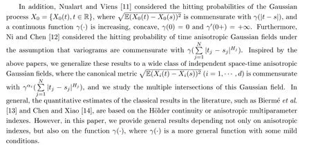
(2)Compared with the conditions in Ni and Chen[12],it is not difficult to find thatγαi(·)is commensurate withγ(·) in Ni and Chen [12].Moreover,αishows the anisotropy of a Gaussian field in space.In particular, ifαi= 1,i= 1,···,d, our conditions reduce to the conditions of Ni and Chen [12].

To solve the problem of space anisotropy, Ni and Chen [15] and Chen and Xiao [16] introduced the metricτdefined by

wherex=(x1,···,xd)∈Rd,y=(y1,···,yd)∈Rd.

LetXH={XH(s)∈Rd,s ∈RN1}andXK={XK(t)∈Rd,t ∈RN2}be two independent Gaussian fields.If there exists ∈RN1andt ∈RN2such thatXH(s) =XK(t), we say thatXHandXKintersect.In this paper, the main aim is to consider the multiple intersections for space-time anisotropic Gaussian fields, which mainly includes the following three questions:

(i) Given a Borel setF ∈Rd, when is

Question (i) is related to the hitting probabilities ofX, which has been widely studied for various random fields by many scholars (see Bierm′eet al.[13] and Xiao [9] for more information).After the classical paper of Dvoretzky, Erd¨os and Kakutani [17], the intersection behavior for various stochastic processes was widely researched.Kahane [18, 19] considered Question (ii) for symmetric stable L′evy processes.Khoshnevisan and Xiao [20] gave necessary and sufficient conditions for intersections for certain L′evy processes by applying the potential theory.Question (iii) was considered by Evans [21], Tongring [22], Fitzsimmons and Salisbury[23], and Peres [24] for Brownian motion, by Dalanget al.[25] for a Brownian sheet, by Chen[26], and Chen and Xiao [14] for time anisotropic Gaussian fields, and by Chenet al.[27] and Wang and Chen [28] for time-space anisotropic Gaussian fields.

The main goal of the paper is to consider the hitting probabilities and the multiple intersections of a wide class of independent space-time anisotropic Gaussian fields based on the approach of Bierm′eet al.[13], Chen and Xiao [14], and Ni and Chen [12, 15].In Section 2,we prove upper and lower bounds for the hitting probabilities ofX.In Section 3, we provide answers to Question (ii).In Section 4, Question (iii) is settled by using the results obtained in Sections 2 and 3.

In this paper, we denote the inner product and the Euclidean norm in Rnby〈·,·〉 and|·|,respectively.Thecdenotes an unspecified positive finite constant.The specific constants are numbered asci.j(j=1,2,···) in Sectioni.

2 Hitting Probabilities

In this section, we present answers to Question(i), which concerns the hitting probabilities ofX(t) based on the approach of Bierm′eet al.[13], Xiao [9], and Ni and Chen [12, 15].First,we briefly introduce some basic facts.

LetX={X(t)∈Rd,t ∈RN}be a centered space-time anisotropic Gaussian field defined as in (1.1) in Section 1.For 0＜aj ＜bj ＜∞(j=1,···,N), let

In addition,Cβ′andHβdenote the capacity of orderβ′and theβ-Hausdorffmeasure in the Euclidean metric, respectively.More details on that can be found in Falconer [29].

The following lemma is called a two point local nondeterminism:

Lemma 2.1Let any intervalIbe defined as in (2.1).Then there existsδ ＞0, and for anys,t ∈Isatisfying that|t-s|＜δ, we have that

where the constantc2.1＞0 depends only onI,Handαi.

ProofSince it is a modification of the proof of Lemma 2.2 in Ni and Chen [12], we omit the detailed proof here.□

We now give two lemmas that prove the main theorems of this paper.

Lemma 2.2LetX={X(t)∈Rd,t ∈RN}be a Gaussian field defined by (1.1).For anyM ＞0, there existsδ0＞0 such that, for anys ∈I,r ∈(0,δ0) andx ∈[-M,M]d, we get that

By using the independence ofX1,···,Xd, Lemma 2.2 can be proven.□

Lemma 2.3LetX={X(t)∈Rd,t ∈RN}be a Gaussian field defined by (1.1).Thus,there exists positive constantδ, and for alls,t ∈Iwith|t-s|≤δandx,y ∈Rd, we have that

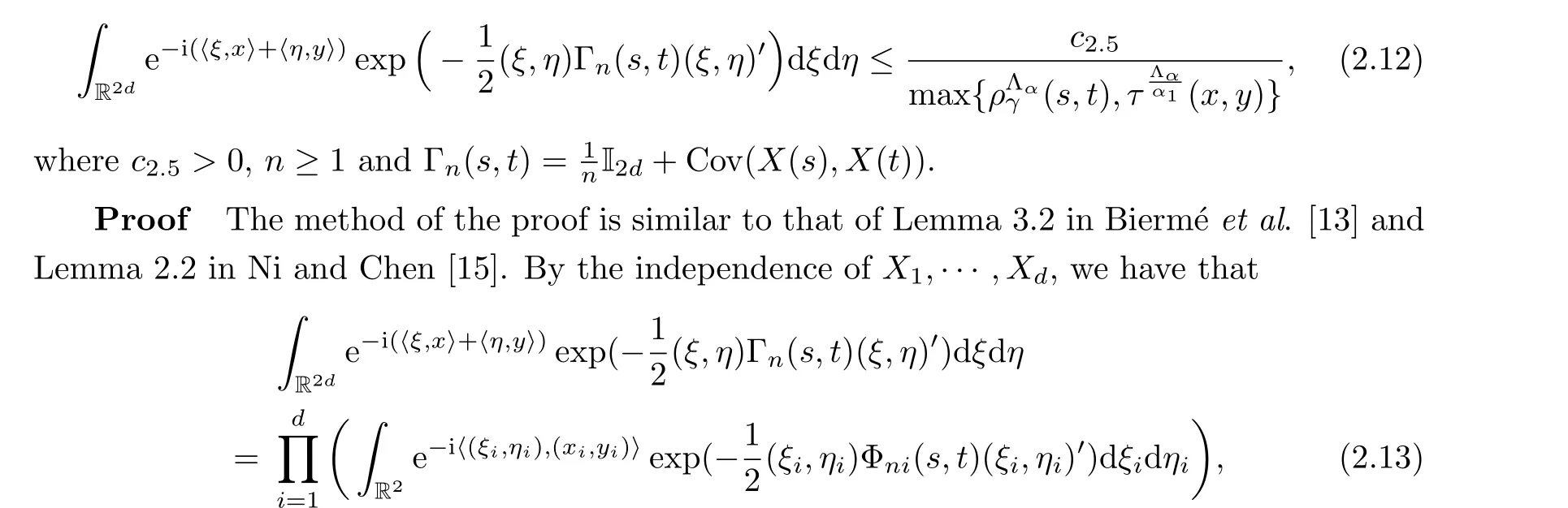
Therefore, we obtain the conclusion (2.12) of Lemma 2.3.□

Next, we will present the main conclusions of this section, which are crucial for studying the multiple intersections.

Theorem 2.4LetX={X(t)∈Rd,t ∈RN}be a Gaussian field defined by (1.1).For all Borel setsE ?IandF ?Rd, we have that

Thus,by(2.19)and the method of Kahane[19],it can be verified that there exists a positive finite measureν0such thatνnconverges weakly toν0, whereν0is carried byX-1(F)∩Eand also satisfies (2.19).Therefore,

Thus, we obtain the lower bound in (2.18).□

Corollary 2.5 LetX={X(t)∈Rd,t ∈RN}be a Gaussian field defined by (1.1).If Λα ≥Q, then, for any Borel setsF ?Rd,

3 Intersections

LetXH={XH(s)∈Rd,s ∈RN1}andXK={XK(t)∈Rd,t ∈RN2}be two independent space-time anisotropic Gaussian fields; that is, let

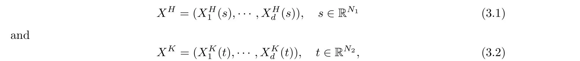
where we have the constant vectorsK= (K1,···,KN2)∈(0,1)N2andH= (H1,···,HN1)∈(0,1)N1.Assume thatXHandXKare defined in the same way as in(1.1),satisfying inequality(1.2) on the intervalsI1?RN1andI2?RN2, respectively.Letγ(·) satisfy Conditions (C1),(C2) and (C3).By Lemma 2.1, we have thatXHandXKsatisfy two points local nondeterminism.

Define a Gaussian fieldZ=(Z(s,t)∈R2d,(s,t)∈RN) by

THERE was once on a time a Fisherman who lived with his wife in a miserable1 hovel close by the sea, and every day he went out fishing. And once as he was sitting with his rod, looking at the clear water, his line suddenly went down, far down below, and when he drew it up again he brought out a large Flounder. Then the Flounder said to him, Hark, you Fisherman, I pray you, let me live, I am no Flounder really, but an enchanted2 prince. What good will it do you to kill me? I should not be good to eat, put me in the water again, and let me go. Come, said the Fisherman, there is no need for so many words about it -- a fish that can talk I should certainly let go, anyhow, with that he put him back again into the clear water, and the Flounder went to the bottom, leaving a long streak3 of blood behind him. Then the Fisherman got up and went home to his wife in the hovel.

Moreover, the above inequality can be obtained from Lemma 3.2.1 of Ni [8].Therefore, the proof is complete.□

Theorem 3.2LetXH={XH(s)∈Rd,s ∈RN1}andXK={XK(t)∈Rd,t ∈RN2}be two independent anisotropic Gaussian fields defined as above.Thus, for all Borel setsE1?I1andE2?I2, there exist positive constantsc3.1andc3.2, such that

ProofSince the events{XH(E1)∩XK(E2)/=?}and{Z(E1×E2)∩{0}/=?}are equivalent,we can use Theorem 2.4 to get the conclusion(3.6),withE=E1×E2andF={0},as long as we can verify the following two conditions:

(2) there existδ ＞0 andc ＞0 for all (s,t),(s′,t′)∈Isatisfying|s-s′|＜δand|t-t′|＜δsuch that we have that

wherei=1,···,dand the last inequality of above is derived from Lemma 3.1.Thus, we have proven thatZsatisfies condition (2).This completes the proof.□

In particular, we will consider the case ofE1=I1,E2=I2.Let

4 Multiple Intersections

Next, we will answer Question (iii).We continue to use the same setting and assumptions as in Section 3.Assume thatQ=QH+QKandN=N1+N2.

Define a Gaussian fieldY={Y(s,t)∈R2d,(s,t)∈RN}byY(s,t) = (XH(s),XK(t)),(s,t)∈RN.Then Question (iii) is equivalent to the following: for ～F={(x,x):x ∈F}?R2d,when is

Theorem 4.1 LetXH={XH(s)∈Rd,s ∈RN1}andXK={XK(t)∈Rd,t ∈RN2}be two independent anisotropic Gaussian fields defined by (3.1) and (3.2), respectively.For all Borel setsE1?I1,E2?I2andF ?Rd, there exist constantsc4.1＞0,c4.2＞0 depending only onI1,I2,F,H,Kandαsuch that

Assume thatλ1andλ2are the restrictions for normalized Lebesgue measures onI1andI2,respectively.Thus,μ=λ1×λ2×σis a probability measure onI1×I2×F.Next, we only need to verify that

By (4.14) and Fubini’s theorem, it is enough to proof that

ProofThe corollary can be proven by modifying the proof of Corollary 3.3, so we omit it the proof here.□

Conflict of InterestThe authors declare no conflict of interest.