
Liutex core line and POD analysis on hairpin vortex formation in natural flow transition *
2020-04-02 03:55SitaCharkritPushpaShresthaChaoqunLiu
水動力學研究與進展 B輯 2020年6期
Sita Charkrit , Pushpa Shrestha, Chaoqun Liu
1. Department of Mathematics, Maejo University, Chiang Mai, Thailand
2. Department of Mathematics, University of Texas at Arlington, Arlington, Texas 76019, USA
Abstract: In this study, the new method of the vortex core line based on Liutex definition, also known as Liutex core line, is applied to support the hypothesis that the vortex ring is not a part of the Λ-vortex and the formation of the ring-like vortex is formed separately from the Λ-vortex. The proper orthogonal decomposition (POD) is also applied to analyze the Kelvin-Helmholtz (K-H) instability happening in hairpin ring areas of the flow transition on the flat plate to understand the mechanism of the ring-like vortex formation.The new vortex identification method named modified Liutex-Omega method is efficiently used to visualize and observe the shapes of vortex structures in 3-D. The streamwise vortex structure characteristics can be found in POD mode one as the mean flow. The other POD modes are in stremwise and spanwise structures and have the fluctuation motions, which are induced by K-H instability.Moreover, the result shows that POD modes are in pairs and share the same characteristics such as amplitudes, mode shapes, and time evolutions. The vortex core and POD results confirm that the Λ-vortex is not self-deformed to a hairpin vortex, but the hairpin vortex is formed by the K-H instability during the development of Lambda vortex to hairpin vortex in the boundary layer flow transition.
Key words: Liutex vector, Liutex core line, proper orthogonal decomposition (POD) analysis, K-H instability, Lambda vortex,Hairpin vort
Introduction
Vortices are considered as a major of turbulent flows. Vortices can be characterized by structural shapes, which can be observed by experiments or simulations. It is well-known that spanwise vortex(parallel to the y-axis), -Λshaped vortex, and hairpin vortex commonly appear in flat plate flow transition in both experiments and direct numerical simulation (DNS) simulation for natural flow transition,while the bypass transition may not have such a process.The hairpin vortex typically consists of three parts: (1)two counter-rotating legs, (2) a ring-like vortex known as the vortex head, which is always in Ω-shape, (3)necks that connect the head and two legs. The formation of vortex is an important topic to study the physics of vortex and turbulence development. One way to get a better understanding of turbulence is to study how one type of vortex evolves into another type especially in the flow transition. In a natural flow transition, it was found in the studies[1-2]that the mechanism of spanwise vortex becomes-Λvortex is due to the vortex filaments redirection and reorganization. The two roots of a -Λvortex known as two legs are two counter-rotating centers containing opposite signs of streamwise vorticity. After the -Λ shaped vortex is formed, the hairpin vortex appears.Then, multiple vortex rings are formed one by one. In this paper, we only discuss the natural flow transition and skip the bypass flow transition.
For the mechanism of the -Λvortex becoming the hairpin vortex, many researchers believe that the formation of the vortex ring is caused by vorticity self-deformation. Hama[3]and Hama and Nutant[4]studied the formation and development of -Λshaped vortices by applying means of flow visualization in water. Knapp and Roache[5]also concluded that the Lambda vortex deforms into the hairpin vortex by using smoke visualizations in air. Moin et al.[6]gave an explanation about the mechanism for the generation of ring-like vortices in turbulent shear flows by using Biot-Savart law for 2-D and DNS for 3-D. The results in Ref. [6] demonstrated that the -Λvortex becomes ring-like vortex by self-deformation as shown in Fig. 1.Although the calculation of vortex layer in the study[6]could be correct, the concept of vortex definition could be incorrect as the vorticity lines and tubes were considered to represent vortex since vorticity and vortex are two different vectors which are not correlated. This would lead to a misunderstanding about the hairpin vortex formation through the self-deformation of the Lambda vortex.

Fig. 1 Sketch of vorticity lines at a different time
Since Helmholtz[7]introduced the concepts of vorticity filament and tube in 1858, many people have considered using vorticity tubes/filaments to represent vortex. The vorticity is mathematically defined by velocity curl, ω=?×V . However, this concept could cause many misunderstandings, which is one of the major obstacles in turbulence research. Vorticity tubes cannot represent vortices in general, especially in viscous flows. Robinson[8]demonstrated that the actual vortices can be weak even though the vorticity is strong near the wall surface areas. Since then, many vortex identification methods have been introduced to capture the vortex structures. One of the popular and well-known vortex identification criteria named as 2λ[9]has been widely applied by the computational fluid dynamics community. However, the physical meaning of2λ is not very clear and the iso-surface of2λ could present some fake vortex structures depending on the selection of the thresholds.Therefore, use of λ2-criteria may not be appropriate to visualize vortex structures.
In 2014, the combination of2λ and vortex filament was applied by Yan et al.[1], Liu et al.[2]to study the mechanism of the late stages of flow transition in a boundary layer at a free-stream Mach number of 0.5 using DNS simulation. In those papers,the difference between the vortex filament that Helmholtz defined, and the natural vortex was also pointed out. It is reported that the -Λvortex and subsequent legs of the hairpin vortex are not vorticity tubes since a vorticity tube cannot be penetrated by any vorticity lines. As a result, they gave a counterexample to the previous conclusions of the self-deformation of Lambda vortex to a hairpin vortex.They concluded that the vortex ring is not a part of the original -Λvortex but is formed separately, and the formation of a -Λvortex into a hairpin vortex with a vortex ring is caused by the shear layer instability or so-called K-H instability. The mechanism of the formation of a -Λvortex to a hairpin vortex caused by K-H instability will be revisited in Section 3.
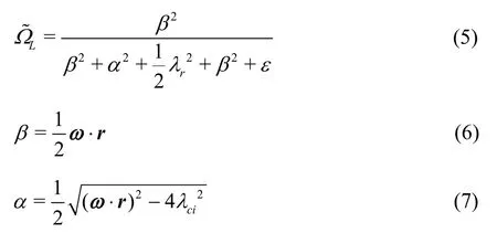
Recently, Liu et al.[10-12], Gao and Liu[13-14]introduced a new physical quantity of “Liutex” to represent a rigid rotation part of fluid flow which is able to show the local direction of rotation. In the previous discussion, it is already mentioned why vortices cannot be represented by the vorticity in general. Vorticity should be decomposed into two parts, a rotational part, and a non-rotational part. In other words, vorticity consists of Liutex (R) and the antisymmetric shear (S), which can be described by the mathematical expression ω=?×V=R+S .Moreover, the velocity gradient tensor can be decomposed to a rotational part (R) and a nonrotational part (NR), i.e., ?V=R+NR which is called UTA R-NR decomposition. Liutex vector is the rotational part of vorticity without shear contamination and defined by R=Rr, where r is the real eigenvector of the velocity gradient tensor?v and R is the rotation strength (twice of the rigid-body angular speed). Wang et al.[15]recently proposed an explicit formula of the magnitude R as follows

where ω is a local vorticity vector,ciλ is an imaginary part of the complex eigenvalue of ?v. As the above description, Liutex can provide the rotation axis, the rigid-body angular speed, and the tensor form.Besides, Liutex is local, accurate, unique, systematical,and Galilean invariant. Since vortices are recognized as the rotational motion of fluids, it is more reasonable to represent vortex by Liutex vector than using vorticity or any other vortex identification criteria.The introduction of Liutex is one of the major achievements in turbulent research. After the Liutex method is proposed, countless researchers have used Liutex to perform numerous investigations on vortex generation and turbulent research[16-18].
After the Liutex concept was proposed, it is combined with Omega method and the new vortex identification method named as modified Liutex-Omega is developed by Liu and Liu[19]which is a significant improvement over the existing vortex identification methods such as Q-criterion, λ2-criterion. This method is a dimensionless and relative quantity from 0 to 1. The new modified method has many advantages which can be described as follows:(1) It can distinguish the vortex from high shear layers,(2) It is robust and can be set as 0.52 to approximate the iso-surface of vortex structure, (3) It can capture both weak and strong vortices simultaneously.Moreover, Gao et al.[20]has recently introduced the identification of vortex core lines based on Liutex definition. It can represent the vortex rotation axis line,which requires that the Liutex magnitude gradient vector lines align with the Liutex vector. This vortex core line method is threshold-free, which can capture the vortex structure uniquely while other vortex identification methods are strongly threshold-dependent and no one can explain why iso-surface can be applied to represent the vortex structure.
Several tools based on Liutex, namely Liutex magnitude, modified Liutex-Omega method, and vortex core line method, are efficiently used to analyze vortex structures in this paper. Liutex magnitude and modified Liutex-Omega method will be applied in this study to capture the 3-D vortex structures with iso-surface, as well as the vortex core lines based on Liutex will be used to analyze the formation of a ring-like vortex.
Furthermore, like the result in the studies[1-2], it is shown that the -Λvortex is not self-deformed to a hairpin vortex (also shown by the vortex core line in our study) but is formed by K-H instability. The proper orthogonal decomposition (POD) is also used to analyze the ring-like vortex formation in the natural flow transition. It has been applied to support the studies[1-2]that the formation process of a -Λvortex to a hairpin vortex is caused by the K-H instability.
POD has been widely applied to extract the coherent structure of fluid flows to understand the complexity of turbulent flow. The original POD was introduced by Lumley[21]in 1967 to investigate the turbulent flow. The other version, snapshot POD, was introduced by Sirovich[22]in 1987 to optimize the computation. In the POD method, the flow structure is decomposed into orthogonal modes ranking by their kinetic energy content and it can be decoupled into the spatial and temporal modes in different applications.For example, a mixing layer downstream on a thick splitter plate obtain from DNS was examined by POD[23]. POD was also applied to turbulent pipe flow[24-25]. The vortex structure in an micro vortex generator (MVG) wake was analyzed by POD in the study[26]. POD has also been applied to flow transition.For instance, a transitional boundary layer with and without control was studied by POD[27]. The vortex structure in late-stage transition was analyzed by using the POD[28]. The study[29]also applied POD to investigate asymmetric structures in late flow transition.Recently, Cavalieri et al.[30]conducted the comparative study between spectral proper orthogonal decomposition (SPOD) and resolvent analysis of near-wall coherent structures in turbulent pipe flows where they concluded that the SPOD modes are simply the response modes from resolvent analysis.
Despite all the work on the POD analysis, no one has studied the mechanism of the vortex ring formation in the flow transition by using the Liutex and POD methods yet. Therefore, this paper is proposed to point out two main results by two different strategies: (1)The vortex core line based on Liutex is applied to support the fact that the ring-like vortex is not part of-Λvortex and the -Λvortex is not self-deformed to hairpin vortex, (2) The POD is used to support the theory that the hairpin vortex is formed by K-H instability.
1. Case set up and code validation
The case and code validation have been introduced in our previous researchs[1-2,31]. The DNS code(DNSUTA) was validated by researchers from UTA and NASA Langley. The results were compared to experiments and other’s DNS results[32-33], and the consistency shows that the code is correct and accurate.
Figsure 2 and 3 present the domain of computation and decomposition of the computation domain along the streamwise direction. The grid level is 1 920×128×241, representing the number of grids in streamwise (x), spanwise (y), and wall-normal (z)directions. The grid is stretched in the normal direction and uniform in the streamwise and spanwise directions. The length of the first grid interval in the normal direction at the entrance is found to be 0.43 in wall units (Ζ+=0.43). The flow parameters, including Mach number, Reynolds number, etc. are listed in Table 1. For more detail about case setup and code validation, see Refs. [1-2].

Fig. 2 Computation domain

Table 1 DNS parameters

Fig. 3 Domain decomposition along the streamwise direction in the computational space
2. Modified Liutex-Omega method and vortex core line
In this section, the new concept of the vortex core line and the modified Liutex-Omega method(ΩL) proposed by Liu et al are reviewed.
2.1 Vortex core identification
The vortex structure in the early transition stage visualized by different Liutex magnitudes are shown in Fig. 4. The iso-surface of Liutex magnitude can be visualized by adjusting thresholds. However, the threshold is arbitrary and man-made, and no one knows what the best specific threshold is to represent vortices. This problem may lead to the wrong understanding of the shapes and formations of vortex structures. Note that Figs. 4(a) and 4(b) were drawn by the same DNS data, but different thresholds have given different structures. Likewise, all currently popular vortex identification methods could give different vortex structures using the same DNS data.
Since the vortex core line based on Liutex has been mathematically proposed, it can be used to represent the vortex structure alternatively. According to Refs. [10, 15], some important definitions are introduced as follows:
Definition 1 The rotation vector named as Liutex vector (R) is defined as the local rotation axis and the magnitude (R) of the Liutex vector is defined as the rotation strength (twice the rigid-body angular speed) as follows

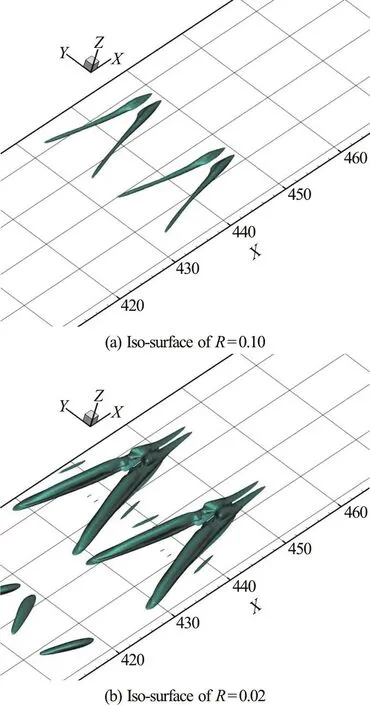
Fig. 4 (Color online) The Λ-vortex at t=6.00T visualized by Liutex magnitude R, where T is the period of T-S wave
where r is the real eigenvector of the velocity gradient tensor ?V. The explicit formula of the magnitude R[15]is given by

where r represents the direction of the Liutex vector.
According to the above definitions, the vortex rotation core line of the flow field is uniquely defined without any threshold requirement. So, the vortex core line method can be used to represent the unique vortex structure. Moreover, the vortex core lines alleviate the burden of choosing a proper threshold.
Figure 5(a) demonstrates Liutex magnitude gradient lines, which concentrate in the center to form the vortex rotation core lines as described by Eq. (4).Moreover, the visualization of a vortex with different thresholds can be represented by the unique vortex core lines as shown in Figs. 6(a) and 6(b). Note that,Figs. 6(a) and 6(b) give a different vortex iso-surfaces,but they have the same vortex core lines which are unique.
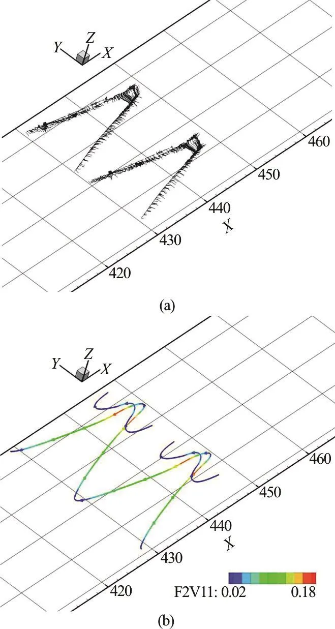
Fig. 5 (Color online) The Λ-vortex at t=6.00T (a) Liutex magnitude gradient without iso-surface, (b) Vortex core lines (red is strong and blue is weak) by Liutex magnitude. F2V11 in above figures is Liutex magnitude represented by R in this research
2.2 Modified Liutex-Omega method
The new vortex identification method named modified Liutex-Omega (LΩ?) method has been proposed in 2019 by Liu and Liu[19]as an effective method to capture vortices. It was developed to improve the Omega method[34]and the published Liutex-Omega method[35-36]and also to replace the previous exiting methods such as Q-criterion[37],λ2-criterion[9].

Fig. 6 (Color online) The Λ-vortex at t=6.00T visualized by Liutex magnitude and vortex core line
Since the introduction of the Omega method in 2016[34], many studies[38-39]have shown that it is more powerful to capture vortices than the existing vortex identification methods. The original Liutex-Omega method is also powerful to visualize vortices but there are some bulging phenomena on the iso-surfaces. As a result, the modified Liutex-Omega method was introduced to resolve some deficiencies in the original Liutex-Omega method.
The modified Liutex-Omega,LΩ?, is defined by
where ω is a local vorticity vector,rλ, λcrand ciλ are a real eigenvalue, a real part of the complex eigenvalue, and an imaginary part of the complex eigenvalue of ?V, respectively. Here, ε is a small positive number used to avoid division by zero or an extremely small number and ε=b (β2-α2)max,where b is a small positive number around 0.001-0.002. In this paper, b is set by b=0.001 and Ω?L=0.52 is applied as an empirical value according to Ref. [40].
3. Ring-like vortex formation
3.1 Observation of Lambda vortex being transformed
to hairpin vortices
It is widely recognized that the evolution of vortex formation in the flow transition can be displayed as in Fig. 7. The vortex structure in Fig. 7 are visualized by the modified Liutex-Omega method.It can be observed that the vortex formation starts with the spanwise vortex, and then the -Λvortex is generated. After the -Λvortex is formed, the ring-like vortex will appear. Then, the multiple hairpin vortices are formed one by one. In the process of evolution of the -Λvortex into the hairpin vortex, which can be seen in the area between x=450 and x=470 in the streamwise direction as shown in Fig. 7 below.There were many studies with experiments and DNS which concluded that the process of -Λvortex becomes hairpin vortex is through the self-deformation.However, this is skeptical and needed to be revisited.
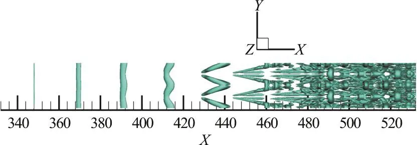
Fig. 7 (Color online) Vortex structures by modified Liutex-Omega method with Ω?L=0.52 at t=13.00T
In our study, the new concept of the vortex core line is applied as a more precise and reasonable way to demonstrate the formation of hairpin vortex without use of iso-surfaces. Therefore, no specified threshold is required. To uniquely represent the vortex strength,the vortex core lines are visualized and colored by Liutex magnitudes as shown in Fig. 8. The -Λvortex is shown with iso-surface at t=6.0T and start to form the first ring in Fig. 8(a). It is clearly shown by the vortex core lines that the rings, which are on top and in the upstream of the tips, are separated from the legs of the -Λvortex as shown in Fig. 8(b). Similarly,at t=6.3T and t=6.5T, the second and third rings are generated separately and independently above the leg of -Λvortex by the visualization of vortex core lines shown in Fig. 8(b). The -Λvortex is likely connected with a ring-like vortex at the tip when it is observed with iso-surface. However, the unique vortex core line demonstrates that the -Λvortex is separated from the ring-like vortex. Therefore, our analyses are consistent with the results of studies[1-2]in 2014 by DNS observation. It can be concluded as follows:
(1) The -Λvortex and ring-like vortex are formed separately and independently.
(2) The ring is not part of -Λvortex.
(3) There is no process that the -Λvortex selfdeforms to a hairpin vortex.
From our investigation of the formation of -Λ vortex by using Liutex core lines, it is found that -Λ vortex does not self-deform into a hairpin vortex,showing consistency with studies[1-2]. So, we can conclude that the self-deformation theory of hairpin vortex formation is produced by a misunderstanding that considers “vortex” as a “vorticity tube”. However,vortex and vorticity are two different concepts and one cannot use vorticity to measure vortex. Since the-Λvortex is not self-deformed to a hairpin vortex,there must be another mechanism of the formation of a hairpin vortex. In the next part, it will be explained that the formation of the -Λvortex to hairpin vortex is caused by the K-H instability.
3.2 Kelvin-Helmholtz instability
The Kelvin-Helmholtz instability occurs when there is a shear-velocity at the interface between two fluid layers. A 2-D vortex ring formation, which is caused by the K-H instability, can be explained as shown in Fig. 9. A low-speed (on the bottom) and a high-speed region (on the top) in opposite directions generate the shear layer as shown in Figs. 9(a), 9(b).Then, the shear layer instability (K-H instability)forms the ring-like vortices by transferring the shear to a pair of rotation cores as in Figs. 9(c), 9(d). In other words, it is a process to transfer non-rotational vorticity or shear to rotational vorticity or Liutex.After that, the pair of rotations becomes one but still has a pair of cores inside the rotation as shown in Figs.9(e), 9(h). Therefore, the paring of vortices is an outstanding symbol of the K-H instability.

Fig. 9 (Color online) Numerical simulation in 2-D on K-H instability. (start from (a) to (h), respectively and the colored lines represent the streamlines)
In the case of pairing in K-H instability, we propose a hypothesis that the vortical structures and some features in the same pairs should be similar.Hence, the POD is applied to show results that support the hypothesis and analyze the ring-like vortex formation. In the next section, the review of the POD method will be first described, and then the results of the POD analysis will be presented.
4. POD analysis of K-H instability in the flow transition
The POD is applied to extract the coherent structure of complex flows and investigate the evidence of the flow transformation. The n snapshots xi=p(ξ,t) are assembled columnwise in a matrix P∈?m×n, which is set from our DNS data by

over 3-D discrete spatial points ξ at times t. In other words, m is a number of spatial points and n is a number of snapshots (time steps). In our case,n?m.
In POD method, the flow field is decomposed into a set of basis functions and mode coefficients as


The reconstructed matrix P in Eq. (13) can also be written into a linear combination as
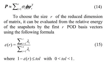
As an application of the POD method, the whole structure can be extracted into r coherent structures.Dimensional reduction can keep the most important modes as a basis. The first mode will be the most dominant energy structure and the last mode will be the least dominant energy structure.
To apply POD in the analysis of the K-H instability, the domain of study is the area where a Λ-vortex transforms into a hairpin vortex. Therefore,the specific area of POD analysis is from ujto x=490 in Fig. 7 displayed above. The POD is applied over 100 snapshots (i.e., 100 time steps) at a time between t=12.51T and t=13.50T to inspect the principal components of the coherent structures. A subzone is extracted to reduce computation complexity. The parameters of the subzone are given in Table 2.
The snapshot ujis taken from each time step which formed the matrix U. The snapshot ujis stacked as follows

where u(i), v(i)and w(i)are velocity fields at t =(12.50+0.01i)T, where i stands for the time steps but not for imaginary number.

Table 2 Parameters of subzone
The POD is applied over 100 snapshots in our study. Therefore, 100 POD modes are obtained. The eigenvalues in the POD method are evaluated and ordered. The POD modes are ranked by the energy content represented by the singular values or the eigenvalues. The results of eigenvalues of all modes are investigated. It is found that two eigenvalues are close to each other in pairs. The eigenvalues of modes 1 and the pairs of the first few modes are presented as shown in Table 3.
In Fig.10, mode 1, which represents the mean velocity (streamwise velocity), is taken out and only the fluctuation modes, which are mode 2 to mode 100,are considered. The eigenvalue of each mode excluding mode 1 and the pairings of eigenvalues can be seen in Fig.10.

Fig. 10 Eigenvalues of mode 2 to 100 indicated the pairs of modes (mode number is shown in Table 3)
By dimensional reduction, the number of modes,r, is chosen by Eq. (15) and shown in Fig. 11. The proper number of modes to reconstruct the vortex structure is 20 modes since it can keep the most cumulative energy as about 100%.

Fig. 11 (Color online) Distribution of ε(r)
The reconstruction performs very well with the first 20 modes comparing to the original flow data.Figure 12 demonstrates that the vortex structures of the original flow and the reconstructed flow of the first 20 modes in two different time steps.
The vortex structures in both original DNS results and reconstructed ones are in different shapes in different time steps as shown in Fig. 12. However,the same shape of vortex structures of each POD mode in different time steps from t=12.51T to t=13.50T is obtained, which is the eigenvector,since the POD mode represents a spatial structure of the flow with the time average.same pair are similar as they have similar eigenvalues and similar eigenvectors.
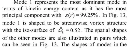
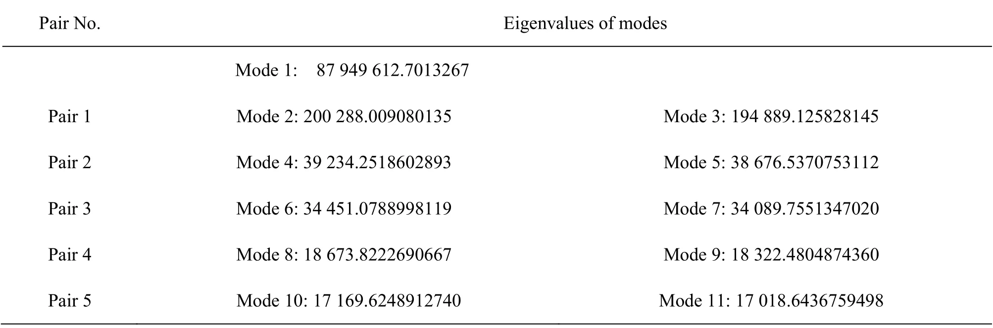
Table 3 Eigenvalues of some modes which occurred in pair
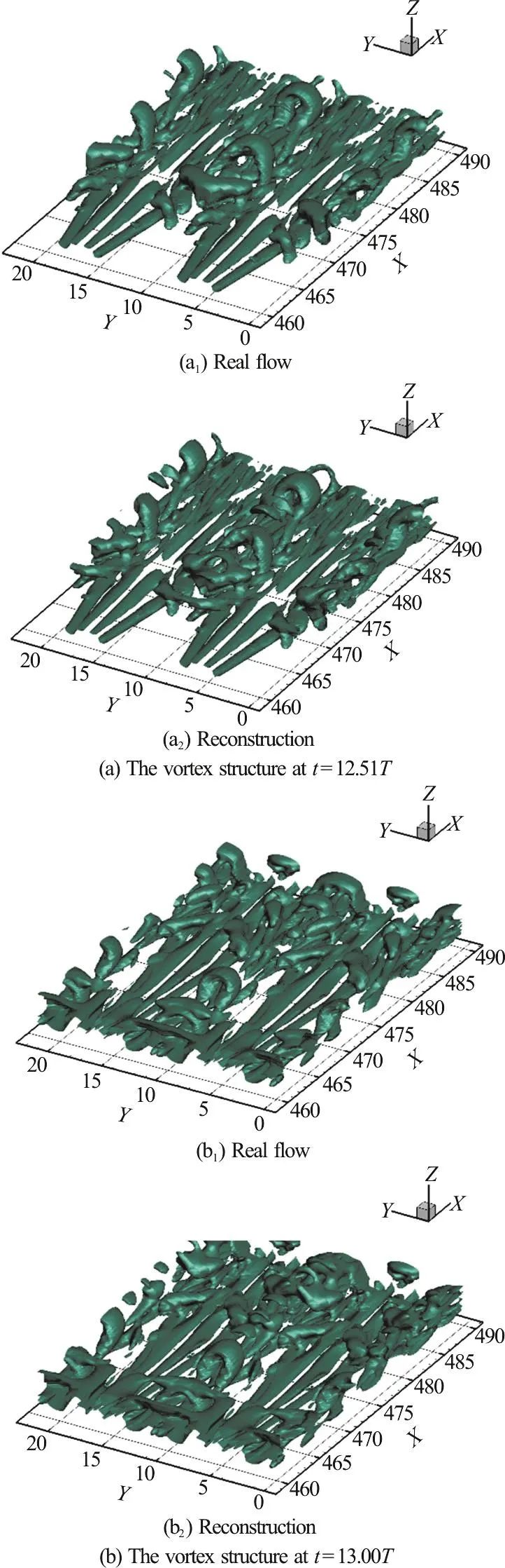
Fig. 12 (Color online) The vortex structure of real flow and reconstruction of the first 20 modes with iso-surface of Ω?L=0.52 with ε=0.001(β2-α2)max
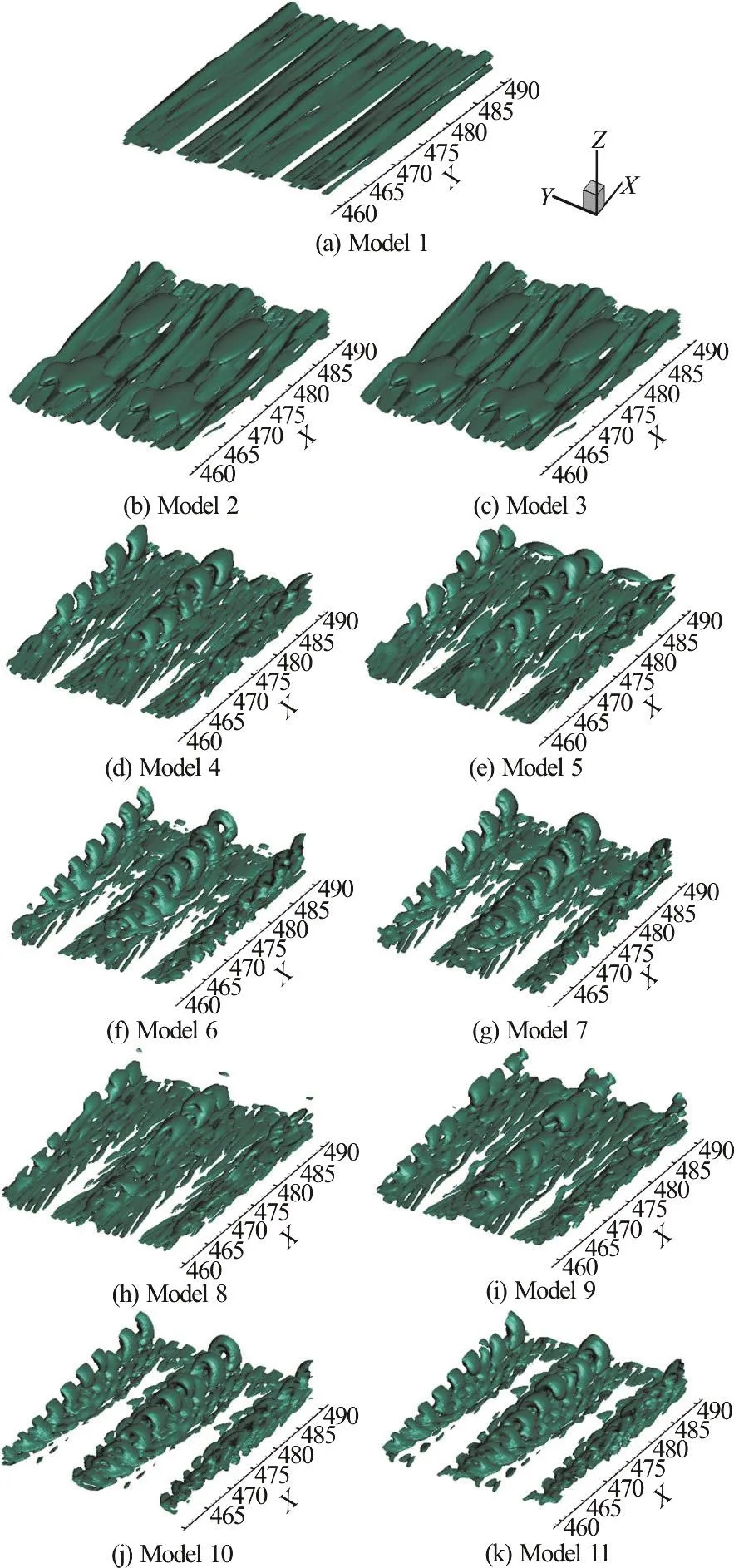
Fig. 13 (Color online) Vortex structures of pairs of modes withiso-surface of ΩL=0.52 with ε=0.001(α2-β2)max
For modes in pair 1, which is a pair of modes 2 and 3, are likely in streamwise characteristic visualized by modified Liutex-Omega method with iso-surface of ΩL=0.52. For the other modes, the vortex shapes are likely dominated by the spanwise structures. As we can see in Fig. 13, the higher modes have smaller spanwise vortex structures and more numbers of rings, which are visualized by the modified Liutex-Omega method.

Fig. 14(Color online) POD time coefficients (y-axis) with mode number (x-axis)
To investigate the fluctuation of flows, the POD time coefficients are applied to demonstrate the periodicities of POD modes. The POD time coefficients are scaled by the singular values of the eigenvectors ψiand they can be obtained from the matrix of temporal structure A=SψTas shown in Eqs. (9) and (11). As we can see in Fig. 14, there is no fluctuation in mode 1 since the graph of the POD time coefficient is likely to be constant. Thus, mode 1 can represent the mean flow. For the other few modes,time coefficients are illustrated in pairs. The similar fluctuations features of modes as periodicities and amplitudes are demonstrated in the same pairs. We can see that the higher modes have higher fluctuations as shown in Fig. 14.
5. Conclusions
The POD is applied to a DNS data with over 100 snapshots to analyze the vortex structure in boundary layer flow transition where the area of a -Λvortex becomes a hairpin vortex because of the K-H instability. The Liutex Core Line method, which is unique and threshold-free, is used for visualization of the vortex structure for the process of Lambda vortex transformation to hairpin vortices. Following conclusions can be made:
(1) Mode 1 is the most energetic mode with leading streamwise structure with no fluctuation.
(2) Modes 2 and 3 are paired and dominated by the stremwise Liutex.
(3) The other modes are dominated by spanwise shapes with fluctuations.
(4) The higher modes have smaller spanwise vortex structures as they are ranked by the eigenvalues.
(5) The smaller eigenvalues in higher modes get smaller-scale structures. The higher modes, which are dominated by the spanwise structures, show more fluctuations.
(6) The POD analysis shows that the eigenvalues and eigenvectors of POD modes are shown in pairs,which is typical in the K-H instability. The same characteristics such as mode shapes and fluctuations are also established in pairs. This evidence is strong proof that K-H instability plays a critical role in the hairpin vortex formation. The K-H instability is always displayed in pairs. Therefore, it can be confirmed that the K-H instability is the main factor of the formation of the hairpin vortex from the -Λ vortex, which transforms the non-rotational vorticity or shear to the rotational vorticity or Liutex.
(7) The theory of self-deformation of the -Λ vortex to hairpin vortex contradicts our DNS observation and analysis and thus may have no scientific foundation because they treat vortex as vorticity.
Acknowledgments
The authors thank the Department of Mathematics of University of Texas at Arlington and Royal Thai Government for the financial support. The authors are grateful to Texas Advanced Computation Center (TACC) for providing CPU hours to this research project. The computation is performed by using Code DNSUTA which was released by Dr.Chaoqun Liu at University of Texas at Arlington in 2009.

- 水動力學研究與進展 B輯的其它文章
- The effects of caudal fin deformation on the hydrodynamics of thunniform swimming under self-propulsion *
- Control of water contamination on side window of road vehicles by A-pillar section parameter optimization *
- Numerical simulation of the effect of waves on cavity dynamics for oblique water entry of a cylinder *
- Reduction of wave impact on seashore as well as seawall by floating structure and bottom topography *
- Applying physics informed neural network for flow data assimilation *
- Experimental analysis of tip vortex cavitation mitigation by controlled surface roughness *