
Evaluation of the Madden–Julian Oscillation in Fengyun-3B Polar-Orbiting Satellite Reprocessed OLR Data
2023-01-16 12:06HainanGONGWanchunZHANGLingSUNZizhenDONGPengZHANGLinWANGWenCHENandRenguangWU
Hainan GONG, Wanchun ZHANG, Ling SUN, Zizhen DONG, Peng ZHANG, Lin WANG,Wen CHEN, and Renguang WU,4
1 Center for Monsoon System Research, Institute of Atmospheric Physics, Chinese Academy of Sciences, Beijing 100190
2 National Satellite Meteorological Centre, China Meteorological Administration, Beijing 100081
3 School of Earth Sciences, Yunnan University, Kunming 650500
4 School of Earth Sciences, Zhejiang University, Hangzhou 310058
ABSTRACT The present study compares the spatial and temporal characteristics of the Madden–Julian Oscillation (MJO) in Fengyun-3B (FY-3B) polar-orbiting satellite reprocessed outgoing longwave radiation (OLR) data and NOAA OLR data during 2011–2020. The spatial distributions of climatological mean and intraseasonal standard deviation of FY-3B OLR during boreal winter (November–April) and boreal summer (May–October) are highly consistent with those of NOAA OLR. The FY-3B and NOAA OLRs display highly consistent features in the wavenumber–frequency spectra, the occurrence frequency of MJO active days, the eastward propagation of MJO along the equator, and the interannual variability of MJO according to diagnoses using the all-season multivariate EOF analysis. These results indicate that the FY-3B OLR produced by the polar-orbiting satellites is of high quality and worthy of global application.
Key words: Fengyun-3B, outgoing longwave radiation, Madden–Julian Oscillation, multivariate empirical orthogonal function, data evaluation
1. Introduction
The Madden–Julian Oscillation (MJO) is the predominant intraseasonal phenomenon in the tropical regions throughout the year (e.g., Madden and Julian, 1994;Kikuchi et al., 2012; Ling et al., 2017a; Lu and Hsu,2017; Kikuchi, 2020, 2021). MJO has great influences on the tropical weather and climate, including the onset and break of monsoon (e.g., Sultan et al., 2003; Lorenz and Hartmann, 2006; Wheeler et al., 2009; Taraphdar et al.,2018; Liu et al., 2022), tropical cyclone activity (Bessafi and Wheeler, 2006; Klotzbach, 2010, 2014; Jiang et al.,2012; Fowler and Pritchard, 2020), and the El Ni?o–Southern Oscillation (e.g., Zhang and Gottschalck, 2002;Hendon et al., 2007; Shimizu and Ambrizzi, 2016). In addition, MJO also strongly interacts with a wide range of mid–high latitude climate through the atmospheric teleconnections (e.g., Lin et al., 2009; Yoo et al., 2012;Henderson et al., 2017). Generally, MJO has different characteristics in different seasons. It is characterized by a pronounced slow eastward propagation along the equator from the Indian Ocean to Pacific during boreal winter.While MJO is featured by the obviously northward/northwestward propagation of tropical convection over the northern Indian Ocean and western North Pacific as well as eastward movement along the equator during boreal summer (e.g., Wheeler and Hendon, 2004; Kikuchi et al., 2012; Lee et al., 2013; Kikuchi, 2021).
Since the seasonal variation of MJO is of great scientific and social significances, meteorologists have developed different approaches with various degrees of complexity to define an all-season MJO (Kikuchi et al.,2012). The simplest method perhaps is to extract an MJO fluctuation of a single variable at a particular location to describe the MJO behaviors (e.g., Hendon and Salby,1994; Kim et al., 2017; Wang B. et al., 2019). The most meticulous and comprehensive method is to trace the convective behaviors associated with MJO (e.g., Wang and Rui, 1990). Furthermore, a conventional and convenient method describing the spatial–temporal variability of MJO is the Eigen techniques (e.g., Wheeler and Hendon, 2004; Pu et al., 2020). For example, the OLR(outgoing longwave radiation)-based extended empirical orthogonal function (EOF) method can be used to represent the typical spatial–temporal characteristics of all-season MJO (Kikuchi, 2020, 2021; Wang et al., 2022). Another example of Eigen techniques is the multivariate EOF analysis. A pioneering work of the method is Wheeler and Hendon (2004) that introduced an all-season MJO index for real-time monitoring by combining near-equatorially averaged OLR and zonal winds at 850 and 200 hPa in the multivariate EOF analysis. In any definition, the OLR is widely used to describe the convective behavior of MJO (Kikuchi et al., 2012). Thus, a better observation and estimation of the global OLR is required for a more accurate reproduction of MJO.
OLR is defined as the total outgoing radiation flux emitted from the earth’s surface and atmosphere at infrared wavelength, which is often used as a proxy for convection in tropical and subtropical regions (Wu and Wang, 2000; Wang and Yan, 2021). Several instruments onboard meteorological satellites provide the global observation of OLR including the broadband and narrowband radiometers. According to Wang and Yan (2021),the broadband radiometers include the Earth’s Radiation Budget (ERB) instrument onboard the NOAA and NIMBUS (series of meteorological satellites) and the Clouds and the Earth’s Radiant Energy System (CERES) instrument onboard the Aqua and Terra satellites, whereas the narrowband radiometers contain the Advanced Very High Resolution Radiometer (AVHRR) instrument onboard the NOAA satellite, the Visible Infrared Spin Scan Radiometer (VISSR) instrument onboard the Geostationary Operational Environmental Satellite (GOES) and Fengyun-2 (FY-2) satellites of China. Among these, the global OLR data obtained from the AVHRR radiometer onboard the NOAA series satellites have the longest history and have been widely used to investigate various weather and climate phenomena (Lee et al., 2013; Wang B. et al., 2019).
Currently, most global estimates of OLR are derived
from polar-orbiting satellites with twice observations per day per satellite (Ellingson and Ba, 2003). The Chinese polar orbiting meteorological satellites consist of FY-1 series and FY-3 series satellites. FY-1 is the first generation polar-orbiting satellites of China, which was launched in July 1988. FY-3 series satellites launched in May 2008 are the second generation polar-orbiting satellites with large development and improvement from FY-1 series satellites (Xian et al., 2021). The Visible Infrared Radiometer (VIRR) onboard the FY-1 and FY-3 polar-orbiting series satellites are used to detect the shortwave and longwave radiation reflected and scattered by the earth’s atmospheric system (Wu and Yan, 2011;Yang H. et al., 2011, 2012; Yang J. et al., 2012; Sun et al., 2013; Xu et al., 2015), respectively, and thus provide available OLR data. It has been reported that the FY OLR data reprocessed by the polar-orbiting satellites is able to well describe various climate phenomena (Yang et al., 2020; Wang and Yan, 2021), whereas limited studies have been carried out to evaluate the all-season MJO behaviors. This study provides an evaluation of the MJO behaviors in FY OLR data by a comparison against those in NOAA OLR. The descriptions of the data and methods are presented in Section 2. Section 3 evaluates the MJO behaviors in theFY-3Bpolar-orbiting satellites reprocessed OLR data. Finally, the summary and discussion are provided in Section 4.
2. Data and method
2.1 Data
TheFY-3Bsatellite is the earth’s observation polar-orbiting satellite of China with high spectral resolution that can provide multi-spectral observations under all weather conditions (Wang and Yan, 2021). In the present study,the daily OLR data in theFY-3Bsatellite is provided by the National Satellite Meteorological Center (NSMC) of the China Meteorological Administration (CMA) with a horizontal resolution of 0.5° × 0.5° and covering the period 2011–2020. Differing from the operational version,the new versionFY-3BOLR data is produced from the re-calibratedFY-3Bhistorical data. The homogeneity and harmonization of the dataset have been improved. The daily global OLR data obtained from the AVHRR radiometer onboard the NOAA series satellites (Liebmann and Smith, 1996) are applied in the evaluation of the performance of theFY-3BOLR data. The NOAA OLR data have been widely used to investigate various climate phenomena over 40 yr (Xu and Guan, 2017; Wang L. et al., 2019), thus being a good reference to validate theFY-3BOLR data. Daily mean atmospheric variables are derived from the 6-hourly data of the newly released fifth generation of the ECMWF Reanalysis (ERA5) dataset(Hersbach et al., 2020). Both NOAA and ERA5 datasets have a horizontal resolution of 2.5° × 2.5° grid and cover the period from 1979 to the present. In order to better compare theFY-3Bdataset with NOAA, theFY-3BOLR is converted to the same resolution as NOAA OLR using the bilinear interpolation.
2.2 Method
In this study, an all-season MJO is identified by using the multivariate EOF analysis of variables that have been bandpass filtered to intraseasonal periods (Wheeler and Hendon, 2004; Clivar Madden–Julian Oscillation Working Group, 2009). The multivariate EOF is used because this method can present well the convection–circulation coupled phenomenon and the baroclinic structure of MJO at the same time by using OLR and zonal winds at 850 and 200 hPa, which will not only allow a comparison between theFY-3Band NOAA reprocessed OLR datasets directly, but also allow an assessment on the coupling betweenFY-3BOLR and newly atmospheric circulation datasets. The process consists of four steps. First, the unfiltered anomalies are computed by subtracting the climatological daily mean from all years of data (i.e.,2011–2020). Second, the 20–100-day bandpass filtered anomalies are obtained by using a 201-point Lanczos filter (Duchon, 1979), which has half power points during 20- and 100-day periods. The Lanczos filter is used in the study because only two inputs are required in the filtering process including the number of weights and the value of the cutoff frequency, both of which can be controlled independently. It results in a simplicity of calculating bandpass filtering and make the Lanczos filtering an attractive filtering method. Other filter such as a Butterworth bandpass filtering is also used, and the result remains consistent (omitted). Third, the combined fields of near-equatorially averaged (15°S–15°N) 850- and 200-hPa zonal winds, and satellite-observed OLR data are combined in the multivariate EOF, and the projections of the bandpass filtered daily anomalies onto the first two EOF models are used to obtain the principal components(PCs) time series. In the EOF analysis, the covariance matrix is used to compute the eigenvector, and each field is normalized by its variance. The normalization ensures that each field has nearly equal contributions to the variance of the combined fields (Clivar Madden–Julian Oscillation Working Group, 2009). Fourth, the resultant PCs are used to generate the MJO life cycle composites by the corresponding phase space, and the coherence squared and phase between the PCs are calculated to de-
termine the fidelity of MJO’s eastward propagation. In addition, the seasonality in the MJO is featured by a latitudinal migration across the equator between two peak seasons. The primary peak season is in boreal winter, and the secondary peak season is in boreal summer (Zhang and Dong, 2004). Thus, we perform our diagnostics of MJO for two broadly defined seasons including the boreal winter (November–April) and boreal summer(May–October) during the shared period of two OLR data from 2011 to 2020. The results are similar if the shorter months are used to define the seasons (i.e.,December–March as winter and June–September as summer; figure omitted).
3. Results
3.1 Preliminary evaluation of MJO
Mean states of OLR during the extended winter(November–April) and the extended summer (May–October) are presented in Fig. 1. The spatial distributions of climatological mean OLR are quite similar in the two datasets. In boreal winter, the climatological OLR has local maximums over the northern Indian Ocean, northwestern Pacific, and eastern South Pacific, and local minimums over the Maritime Continent (Figs. 1a, c). It is known that a lower OLR represents a stronger tropical convection. Hence, the above result indicates that a stronger wintertime convection occur over the Maritime Continent , which may be related to the active region of MJO (Kikuchi et al., 2012). In boreal summer, the local OLR values move slightly to the north since the seasonal movement (Figs. 1b, d). In comparison with two OLR datasets, the climatological OLR over the Indo-Pacific sector has tiny differences in both seasons (Figs. 1e, f)and their spatial correlation are 0.994 and 0.991 for boreal winter and summer, respectively. The results indicate a well reproducibility of the OLR climatology inFY-3Bseries satellites. However, some large differences can be found in the extratropics (Figs. 1e, f). The changes in extratropical OLR sometimes represent the surface temperature not the convection variations due to a lack of cloud, and may not be related to MJO.

Fig. 1. Climatology of seasonal mean OLR (shade; W m?2) for (a, c, e) November–April and (b, d, f) May–October during 2011–2020 in (a, b)FY-3B, (c, d) NOAA datasets, and (e, f) difference between two datasets.
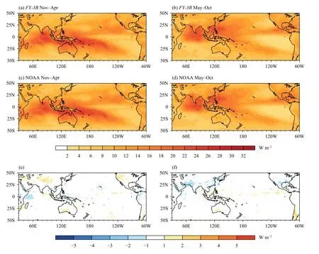
Fig. 2. As in Fig. 1, but for standard deviation of 20–100-day filtered OLR anomalies (shade; W m?2).
Figure 2 shows the standard deviation of 20–100-day filtered OLR anomalies associated with the MJO variability inFY-3Band NOAA datasets. Large variability is observed over the tropical Indian Ocean, Maritime Continent, and tropical western Pacific with the local maximum south of the equator during boreal winter (Figs. 2a, c).Those during boreal summer are over the northern Indian Ocean and western North Pacific (Figs. 2b, d). The results are consistent with the previous studies (Kikuchi et al., 2012; Lee et al., 2013) , and indicate that MJO is an active intraseasonal phenomenon south of the equator in winter and north of the equator in summer. The spatial correlation between the distributions of MJO variability in two OLR datasets are very high with the correlation coefficients at 0.990 and 0.987 for winter and summer,respectively. The difference in the magnitude of MJO variability over the Indo-Pacific sector is negligible betweenFY-3Band NOAA satellites (Figs. 2e, f), where the MJO is active. Hence, the comparison between the two OLR datasets indicates a well-done expression of MJO variability inFY-3Bsatellites.
Figure 3 shows the wavenumber–frequency power spectra of 15°S–15°N averaged OLR, which provides a convenient metric of the MJO characteristics. By definition, positive frequency represents the eastward propagation, whereas negative frequency represents the westward propagation. For standing oscillations, equal amount of power is expected in eastward and westward directions (Clivar Madden–Julian Oscillation Working Group, 2009). A concentration of eastward power is observed during 20–100-day periods with zonal wavenumbers 1–3, and a clear standing oscillation is seen at a period more than 100 days (Figs. 3a–d). The eastward power is about three times that of westward power at the intraseasonal frequencies of MJO. A comparison between boreal winter and boreal summer shows that both seasons exhibit qualitatively similar and consistent spectral characteristics except their amplitudes. These results are highly consistent in two OLR datasets (Figs. 3a–d).
Furthermore, the MJO is closely associated with the convectively coupled equatorial waves (CCEWs) within the context of multiscale interaction. On the one hand,the MJO exerts strong modulation on the CCEWs that primarily through changing the environment moisture and circulation fields (e.g., Roundy, 2008; Khouider et al., 2012; Guo et al., 2014). On the other hand, the CCEWs feed back to the MJO through the upscale transports of momentum, temperature, and moisture (e.g., Liu and Wang, 2013; Guo et al., 2015). The two-way interactions between MJO and CCEWs are the fundamental features of MJO. Hence, the capability ofFY-3Breprocessed OLR data in depicting the CCEWs should be further evaluated. Figure 4 presents the wavenumber–frequency spectrum of the symmetric component of daily OLR over the tropics (15°S–15°N). Note that power spectrum is shown as the ratio of raw spectrum to the background spectrum. The diagram of zonal wavenumber and frequency, dominant modes shown by spectrum peaks are eastward MJO and Kelvin wave, and westward equatorial Rossby wave (n= 1 ER) and inertiogravity wave (n= 1 WIG). This is consistent with previous studies (e.g., Wang and Chen, 2016; Wang L. et al.,2019). The results highly agree with theFY-3Band NOAA daily OLR datasets, and their spatial correlation coefficient is 0.925, thus indicating the reliability ofFY-3BOLR data to describe the MJO-associated tropical features.
3.2 Multivariate EOF defined MJO
As described in Section 2.2, MJO can be defined by the multivariate EOF analysis (Wheeler and Hendon,2004; Clivar Madden–Julian Oscillation Working Group,2009). The spatial structures of the leading two EOFs of the combined fields for OLR, 850- and 200-hPa zonal winds are presented in Fig. 5. Together, the first two EOF models explain 44.3% and 44.1% of the overall variance inFY-3Band NOAA datasets, respectively,which are well separated from the remaining EOFs based on the North criterion (North et al., 1982). Calculation of the variance of individual fields accounted for by each EOF is also exhibited, and both OLR datasets show the similar magnitude of variance.

Fig. 3. Wavenumber–frequency spectral of 15°S–15°N averaged OLR (shade; W2 m?2) for (a, c) November–April and (b, d) May–October during 2011–2020 in (a, b) FY-3B and (c, d) NOAA datasets.
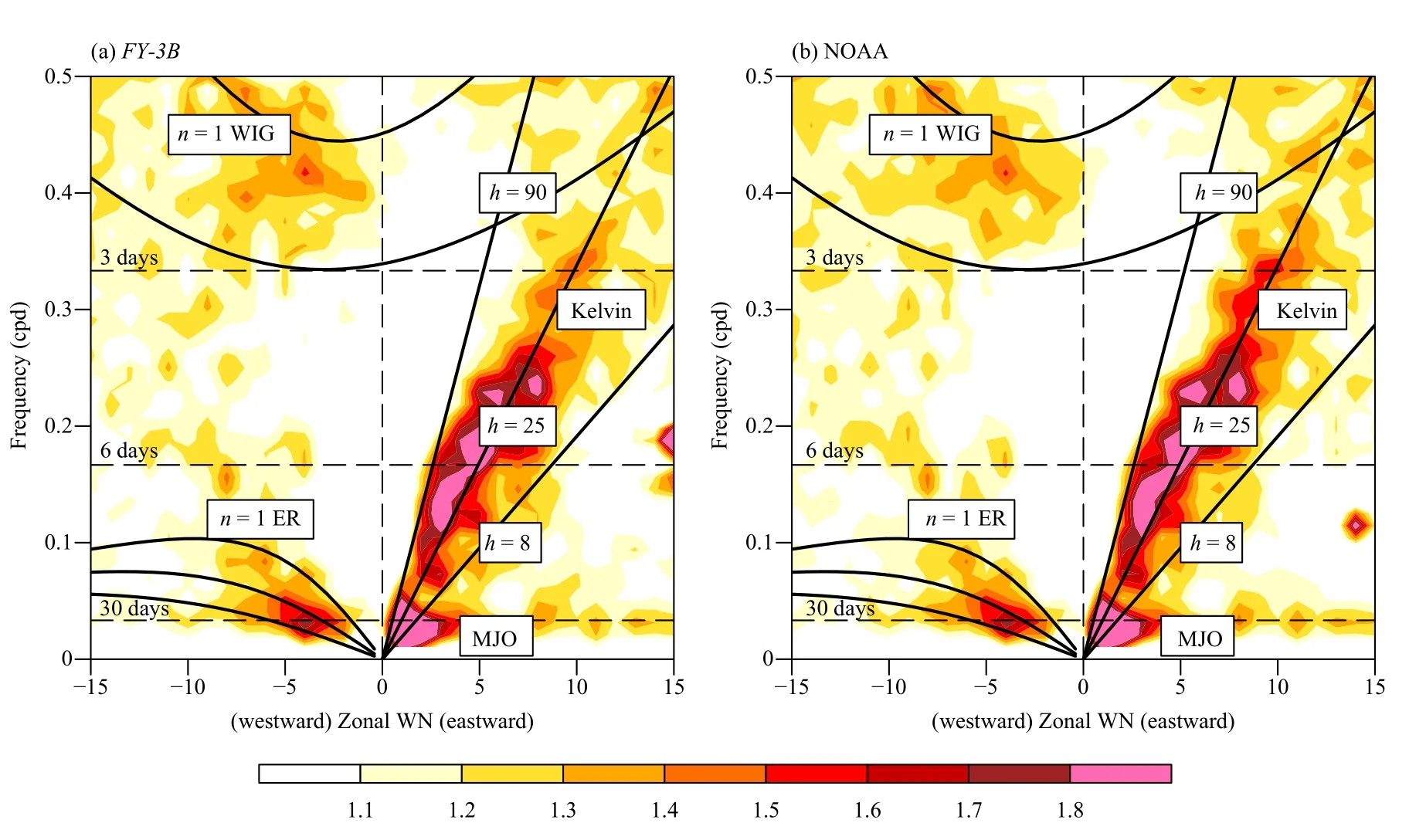
Fig. 4. Wavenumber–frequency power spectrum of the symmetric component of daily OLR from January 2011 to December 2020 between 15°S and 15°N for (a) FY-3B and (b) NOAA satellites, plotted as the ratio between raw OLR power and the power in a smoothed red noise background spectrum. Superimposed are the dispersion curves of equatorial waves for three equivalent depths of 8, 25, and 90 m indicated as the thick solid lines. The signals with positive (negative) zonal wave number propagate eastward (westward). Note that “cpd” in y-axis denotes cycle per day.
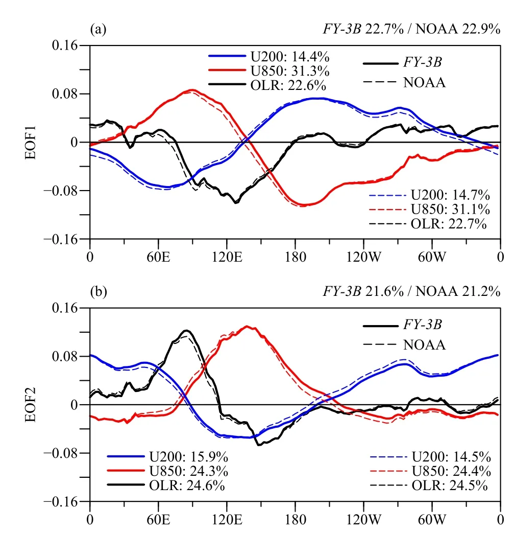
Fig. 5. (a) First and (b) second multivariate EOF modes of 20–100-day filtered and 15°S–15°N averaged OLR (black), and 850-hPa (red)and 200-hPa (blue) zonal winds. The total explained variance by each mode is shown at the top right, and the explained fractional variances of the individual fields at the right of each figure. The thick solid lines and thin dotted lines represent the FY-3B and NOAA datasets.

Fig. 6. Occurrence frequency of significant MJO days as a function of calendar month for the seasonal MJO modes in November–April(blue) and May–October (red) for (a) FY-3B and (b) NOAA datasets.The inner number represents the frequency in each calendar month.
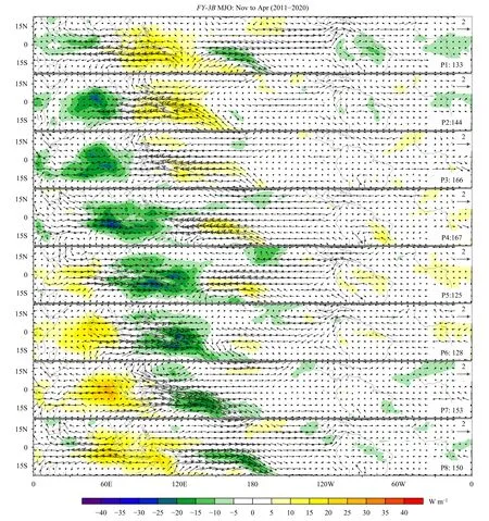
Fig. 7. Composite November–April 20–100-day filtered FY-3B OLR (shade; W m?2) and 850-hPa winds anomalies (vectors; 2 m s?1) as a function of the MJO phase. The composite is based on PC12 + PC22 > 1, and the number of days used to generate the composite for each phase is shown to the bottom right of each panel.
Physically, EOF1 describes the situation when MJO has the enhanced convection over the Maritime Continent accompanied by the low-level westerly wind anomalies on the west side of MJO convection throughout the Indian Ocean, and low-level easterlies on the east side of convection across the tropical Pacific. In the upper level,the zonal wind anomalies are in the opposite direction to those in the low level (Figs. 5a). EOF2 produces the eastward propagation of MJO convection relative to EOF1,and it shows enhanced convection over the western Pacific and suppressed convection over the Indian Ocean(Figs. 5b). The zonal wind patterns are nearly in quadrature with those in EOF1. As a whole, bothFY-3Band NOAA datasets present the consistent MJO structures,and agree well with those obtained from the previous studies (Wheeler and Hendon, 2004; Clivar Madden–Julian Oscillation Working Group, 2009; Ahn et al., 2017).
Figure 6 exhibits the occurrence frequency of significant MJO days among all days in each calendar month during 2011–2020. The significant MJO days are defined as periods when the magnitude of PC12+ PC22exceeds 1, where PC1 and PC2 each have an unit of standard deviation. It is evident that MJO is most active during the winter months (i.e., November–April), while its frequency has a concave-type distribution during the summer months (i.e., May–October) with least activeness in August and September. The result is consistent in both two datasets with a spatial correlation coefficient of 0.997, well exceeding the 99% confidence level based on the two-tailed Student’st-test.
3.3 MJO life cycle
The spatial–temporal structures of MJO during boreal winter and boreal summer are obtained by a composite life cycle within the significant MJO days. In the composite analysis, the phase of the MJO can be related to the inverse tangent of the ratio of PC2 and PC1 (Clivar Madden–Julian Oscillation Working Group, 2009), and the numbers of significant MJO days for each phase are displayed to the right of each panel. During boreal winter, the MJO convection of a growing event is present in the tropical western Indian Ocean in phase 1, while the convection of a decaying event is evident in the tropical western Pacific. At the same time, strong westerly anomalies exist over the Pacific and easterly anomalies over the Indian Ocean. The convection initiated over the western Indian Ocean couples easterly wind anomaly to the east. In the subsequent phases, the growing MJO convection over the Indian Ocean spreads southeastward accompanied by the eastward movement of the 850-hPa wind anomalies. The convective signal first passes through the Maritime Continent and finally reaches a region near the International Date Line (Figs. 7, 8). All those features in the composited MJO life cycle are highly consistent inFY-3Band NOAA OLR datasets, and also in agreement with the early studies (Clivar Madden–Julian Oscillation Working Group, 2009). The spatial correlations of OLR anomalies in each winter MJO phase are all approximately or larger than 0.97 (Table 1).
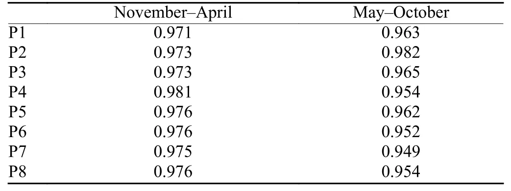
Table 1. Spatial correlations of 20–100-day filtered FY-3B and NOAA OLR anomalies composited during different MJO phases as shown in Figs. 7, 8 and 11, 12
An alternative to look at the MJO life cycle is to use the two-dimensional phase space defined by PC1 and PC2. This presentation is shown for all days in the November–April winter season, and points representing sequential days are joined by a line. Many of the sequential days trace anticlockwise circles around the original day, which signifies a significant eastward propagation of winter MJO. Two separate winters are well identified in 2011/2012 and 2015/2016 (Fig. 9), and their phase spaces are almost the same in the two datasets. Note that the year from 2011 to 2012 is the period of the Dynamics of the MJO/Cooperative Indian Ocean Experiment on Intraseasonal Variability (DYNAMO/CINDY). A special attention should be put on the campaign period from September 2011 to March 2012 to show how well theFY-3BOLR data represents the individual MJO events.Figure 10 shows the longitude–time diagram of the composite OLR anomalies in the 2011/2012 winter. At least two MJO events can be clearly observed during the period,one happens from late November 2011 to middle December 2011, and the other one occurs from late February 2012 to middle March 2012, consistent with those analyzed by Xiang et al. (2015). A comparison between theFY-3Band NOAA OLR datasets shows a large similarity for these two MJO events, and their spatial correlations are 0.963 and 0.975, respectively. Thus, we believe that the OLR data provided byFY-3Bpolar-orbiting satellite can well capture the MJO activity.

Fig. 8. As in Fig. 7, but for the NOAA OLR dataset.

Fig. 9. Phase space points (PC1 and PC2) for all available days for November–April (a) 2011/2012 and (b) 2015/2016 in FY-3B (thick solid lines) and NOAA (thin dotted lines) datasets. Eight defined regions of the phase space are labeled, and the inside circles are considered to signify weak MJO activity. Also labeled are the approximate locations of the enhanced convective signal of the MJO for that location of the phase space.
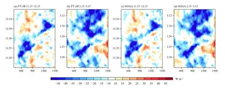
Fig. 10. Longitude–time diagram of the composite anomalies of (a, b) FY-3B and (c, d) NOAA OLR data (shade; W m?2) averaged over 15°S–15°N (a, c) from 15 November to 15 December 2011 and (b, d) from 15 February to 15 March 2012.

Fig. 11. As in Fig. 7, but for May–October 20–100-day filtered FY-3B OLR (shade; W m?2) and 850-hPa winds anomalies (vectors; 2 m s?1) as a function of the MJO phase.

Fig. 12. As in Fig. 11, but for the NOAA OLR dataset.

Fig. 13. Hovm?ller diagrams of MJO phase composited 20–100-day filtered (a, b) FY-3B and (c, d) NOAA OLR datasets (shade; W m?2) during (a, c) November–April and (b, d) May–October averaged between 15°S and 15°N.

Fig. 14. As in Fig. 13, but for the May–October average over (a) IO (60°–80°E) and (b) WNP (110°–130°E).
Figures 11 and 12 show the evolutions of the composited MJO convection and lower-level circulation during the northern summer season. In phase 1, the active MJO convection starts to occur over the central Indian Ocean.The convection develops with time and becomes elongated in phase 2. In phase 3, it split into two parts: one moving eastward and the other moving northward/northwestward in the northern Indian Ocean. The northward propagating MJO convection covers the entire Indian subcontinent in phase 4 and the eastward propagating component reaches the tropical western Pacific, causing an elongated convection band that spreads from the northwest to southeast as a whole in phases 4 and 5. In the subsequent phases, the northward moving convection gradually dissipates over the northern Indian Ocean,whereas the convection over the western Pacific starts to propagate northwestward and weakens with time over the western North Pacific. Meanwhile, the eastward propagating convection, in spite of weaker magnitude,continues to move eastward in the eastern Pacific. Such features of summer MJO are very similar in the two OLR datasets, and the spatial correlations of OLR convection in each summer phase are larger than 0.95 (Table 1). As a result,FY-3Bdataset seemingly reproduces the MJO activity in boreal summer as well.
3.4 Horizontal propagation of MJO
According to the above analysis, a clear eastward propagation of convection exists in the winter MJO, and both eastward and northward movement exist in the summer MJO. In order to visualize the propagating characteristics of the all-season MJO, the hovm?ller diagrams of MJO-phase composited 20–100-day convection are shown in Figs. 13, 14. During boreal winter, the MJO convective signal propagates eastward from Indian Ocean to western Pacific with the reduced magnitude over the Maritime Continent, while the convection normally weakens and vanishes when across the International Date Line (Figs. 13a, c). During boreal summer, the eastward propagating convective signal of MJO still remains obviously, but the convection has an unimodal structure over the Indian Ocean. The magnitude of MJO convection evidently weakens when it reaches the western Pacific (Figs. 13b, d). The spatial correlations of the eastward propagating MJO convection betweenFY-3Band NOAA OLR datasets are 0.997 and 0.996 during boreal winter and boreal summer, respectively.
For the meridional propagation of the summer MJO,there are two significant northward propagating components. One is over the Indian Ocean (IO; 60°–80°E) and the other over the western North Pacific (WNP;110°–130°E) (Figs. 11, 12). Over the Indian Ocean, the MJO convective signal moves northward from the neartropics to the subtropics approximately 15°N (Figs. 14a,c). Over the WNP, the convective signals propagates northward from 5° to 20°N, further north than those over the IO (Figs. 14b, d). However, relative to the northward movement over the IO, the propagation speed is smaller for MJO convection over the WNP. These propagation characteristics are highly consistent in the two OLR datasets with the spatial correlation above 0.99 (0.995 and 0.992). As a result, theFY-3BOLR data capture well the propagating features of the all-season MJO convection.
3.5 Interannual variations of MJO
Interannual variations of the MJO activity are also an important feature to describe the MJO behavior and its possible predictability. In this study, we use the 91-day running mean PC12+ PC22as an index to measure the interannual MJO activity. The major bursts of MJO occur during the early-2012, mid-2013, early-2014, late-2015, early-2016, early-2018, and mid-2019 for both seasons (Fig. 15). The correlation coefficients of the winter and summer indices between theFY-3Band NOAA OLR datasets are 0.989 and 0.991, respectively. Overall, the interannual variation of MJO can be reproduced well inFY-3BOLR dataset.

Fig. 15. Time series of 91-day running mean MJO magnitude represented by the PC12 + PC22 during (a) November–April and (b)May–October. Blue and red lines represent the FY-3B and NOAA OLR datasets.
4. Conclusions and discussion
In this paper, we evaluate the ability ofFY-3BOLR data reprocessed by the polar-orbiting satellite to depict the basic characteristics of the all-season MJO activity during 2011–2020. A multivariate EOF analysis is performed for the 20–100-day filtered combined fields of OLR, 850- and 200-hPa zonal wind anomalies in the tropical belt. The spatial distributions of climatological mean and intraseasonal standard deviation of OLR based onFY-3Bdata are highly consistent those based on NOAA data. Further comparisons show that the OLR data obtained from theFY-3Bsatellite can well reproduce the main features of the all-season MJO, including the wavenumber–frequency power spectra of MJO, lift cycle, propagating characteristics, and interannual variations against the NOAA OLR dataset. Hence, these results indicate that the quality ofFY-3BOLR has reached the international advanced level, and it is very suitable for the research and application in the field of climate variability and climate change. In addition, since theFY-3Bprovides available real-time observation, theFY-3BOLR is worthy of further global application.
In this study, we use theFY-3BOLR data coupled with the atmospheric circulation to describe the MJO activity. However, it should be noted that MJO is a complicated coupling climate phenomenon (Zhang, 2005;Ling et al., 2017b; Chen et al., 2022), which can be also coupled with oceanic processes. Therefore, the coupling between the OLR and oceanic datasets inFY-3Band NOAA are worth to further systematic evaluation to illustrated the dynamic processes of MJO in the further study.
Acknowledgments.The ERA5 data are available online at https://www.ecmwf.int/en/forecasts/dataset/ecmwf-reanalysis-v5, the NOAA OLR data are available online at https://psl.noaa.gov/data/gridded/data.interp_OLR.html, and theFY-3BOLR data are available online at http://www.richceos.cn/record/cn/detail.html?doi=10.121 85/NSMC.RICHCEOS.FCDR.FY3VIRRReproDaily-OLR.FY3.VIRR.L2.GBAL.POAD.GLL.5000M.HDF.20 21.3.V2.
 Journal of Meteorological Research2022年6期
- Journal of Meteorological Research的其它文章
- Record Flood-Producing Rainstorms of July 2021 and August 1975 in Henan of China:Comparative Synoptic Analysis Using ERA5
- Interdecadal Variability of Summer Precipitation in Northwest China and Associated Atmospheric Circulation Changes
- A New Hybrid Machine Learning Model for Short-Term Climate Prediction by Performing Classification Prediction and Regression Prediction Simultaneously
- Surface Weather Parameters Forecasting Using Analog Ensemble Method over the Main Airports of Morocco
- Impacts of the Urban Spatial Landscape in Beijing on Surface and Canopy Urban Heat Islands
- Effect of Using Land Use Data with Building Characteristics on Urban Weather Simulations: A High Temperature Event in Shanghai