
Identification of thermal front dynamics in the northern Malacca Strait using ROMS 3D-model*
2024-02-27 08:27KuNorAfizaAsnidaKuMANSORNurHidayahROSELIPohHengKOKFarizSyafiqMohamadALIMohdFadzilMohdAKHIR
Ku Nor Afiza Asnida Ku MANSOR, Nur Hidayah ROSELI, Poh Heng KOK,Fariz Syafiq Mohamad ALI, Mohd Fadzil Mohd AKHIR
1 Institute of Oceanography and Environment, Universiti Malaysia Terengganu, Kuala Nerus 21030, Malaysia
2 Faculty of Science and Marine Environment, Universiti Malaysia Terengganu, Kuala Nerus 21030, Malaysia
Abstract The thermal front in the oceanic system is believed to have a significant effect on biological activity.During an era of climate change, changes in heat regulation between the atmosphere and oceanic interior can alter the characteristics of this important feature.Using the simulation results of the 3D Regional Ocean Modelling System (ROMS), we identified the location of thermal fronts and determined their dynamic variability in the area between the southern Andaman Sea and northern Malacca Strait.The Single Image Edge Detection (SIED) algorithm was used to detect the thermal front from model-derived temperature.Results show that a thermal front occurred every year from 2002 to 2012 with the temperature gradient at the location of the front was 0.3 °C/km.Compared to the years affected by El Ni?o and negative Indian Ocean Dipole (IOD), the normal years (e.g., May 2003) show the presence of the thermal front at every selected depth (10, 25, 50, and 75 m), whereas El Ni?o and negative IOD during 2010 show the presence of the thermal front only at depth of 75 m due to greater warming, leading to the thermocline deepening and enhanced stratification.During May 2003, the thermal front was separated by cooler SST in the southern Andaman Sea and warmer SST in the northern Malacca Strait.The higher SST in the northern Malacca Strait was believed due to the besieged Malacca Strait, which trapped the heat and make it difficult to release while higher chlorophyll a in Malacca Strait is due to the freshwater conduit from nearby rivers (Klang, Langat, Perak, and Selangor).Furthermore, compared to the southern Andaman Sea, the chlorophyll a in the northern Malacca Strait is easier to reach the surface area due to the shallower thermocline, which allows nutrients in the area to reach the surface faster.
Keyword: regional ocean modelling system; thermal front; Andaman Sea; Malacca Strait; single image edge detection algorithm
1 INTRODUCTION
Thermal fronts are convergence zones between two different water masses with a pronounced horizontal temperature gradient.In the coastal and open oceans, the variability of the air-sea interaction process, such as latent heat, sensible heat, wind intensity, riverine runoff, tidal mixing, and coastal upwelling play important roles in the production of frontal features (Eadie et al., 1994; Davis et al.,2014).Previous studies have shown the important relationship between fronts and the phytoplankton abundance (Mahadevan and Archer, 2000; Lévy et al., 2001; Mahadevan and Tandon, 2006; Sholva et al., 2013), including the potential of phytoplankton bloom in a strong thermal front area (Taylor and Ferrari, 2011).In the area of upwelling or horizontal advection, thermal boundaries are formed by the enrichment of surface water nutrients by the upwelled cold water (Pitcher et al., 2010).These mesoscale activities are productive regions since they are related to high nutrients and chlorophylla(Chla).In a frontal zone, this cold and highlynutrients water is separated by warm and lessnutrients water on the other side.With climate change, the heat absorbed by the ocean is increasing and causing the sea surface temperature (SST) to increase.As the SST increase, it will alter the air-sea interaction process, which causes changes in the thermal front formation and thus affects the primary production in the ocean (Roxy et al., 2016).
The understanding of the ocean has substantially improved with the development of remote sensing,satellites, numerical ocean modelling, and other marine observational platforms.These methods had been used to identify ocean features such as eddies,gyres, current circulation, upwelling/downwelling zones, and fronts which has improved our perception of the global oceans (Traykovski and Sosik, 2003).The Advanced Very High-Resolution Radiometer(AVHRR) sensor provided by National Oceanic and Atmospheric Administration (NOAA) satellites has been widely used and shown to be beneficial in determining the effect of temperature on productivity(Solanki et al., 2001; Strong et al., 2004; Skirving et al., 2006; Mohanty et al., 2013).Stretta (1991) used remote sensing datasets (SST, Chl-aconcentrations,sea surface winds, geostrophic current) in identifying fish aggregation sites across the world oceans.Similar efforts have been done to assist fishing communities in decreasing labour, risk, search time,and fuel consumption associated with fishing operations.Such attempts extend back to the 1990s when initial research was conducted in the northeast Arabian Sea due to the least amount of cloud cover throughout the course of a year (Solanki et al., 2001,2003, 2005, 2008; Nayak et al., 2003; Dwivedi et al.,2005).These efforts were later used in operational service.The results of this service, known as Potential Fishing Zone Advisories, have also been validated and reported adequately (Subramanian et al., 2014).Meanwhile, Daulay et al.(2019) and Ilhamsyah et al.(2018) have used satellite images to determine thermal front and high productivity areas in the eastern Indian Ocean and the southern Andaman Sea respectively.The shortcoming of using remote sensing and satellite images in identifying fronts is these tools could not provide deep layers of information.To address these shortfalls, this research employed a 3D numerical modelling that can be served as an alternating tool to describe the thermal front since it is able to provide data for a long-term period, bigger region, and subsurface area.
Regional Ocean Modelling System (ROMS) is used to determine the thermal front dynamics in the area between the southern Andaman Sea and northern Malacca Strait (Fig.1).The single image edge detection(SIED) algorithm is used to detect the fronts whereas previous research has demonstrated the relationship between physical and biological parameters using this method (Cayula and Cornillon, 1992; Miller,2004).Manual frontal gradient detection, whether for operational or long-term study reasons, is prone to inaccuracy and time-consuming operations.Because most manual front identification is reliant on visual perception and is vulnerable to high uncertainty owing to human error, as a result, image processing techniques have been created to detect fronts from SST and Chl-ameasurement semi-automatically or automatically (Simpson, 1990; Bardey et al., 1999).Such an effort is understood to aid in the demarcation of persistent productive zones since the frontal location is associated with the convergence of the flow of two different types of water (Belkin et al., 2009) where the source of food is accumulated near the fronts, providing a conducive area for spawning,nursing and feeding ground for animals.In addition,due to the convergence flow of water, the floating materials are usually accumulated and trapped near the frontal region, which is important to combat the pollution due to oil spills and garbage.They are important in search and rescue operations since a stricken small craft will remain in the frontal region.Over the long term, the findings of this study are envisaged to provide a foundation for future studies as well as for future ecosystem monitoring systems.
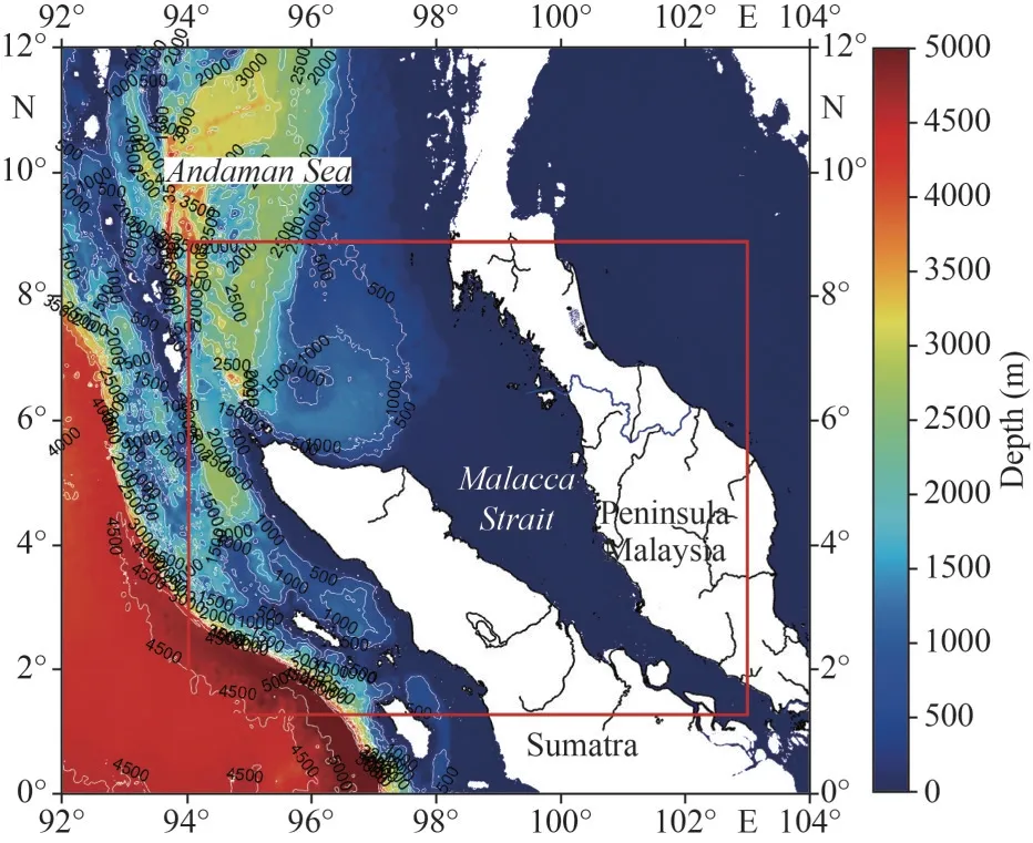
Fig.1 Map and bathymetry of the study region
2 MATERIAL AND METHOD
2.1 Model setting and configuration
The 3D hydrodynamic ocean model employed in the present study is ROMS (http://www.myroms.org) (Haidvogel et al., 2008), which uses hindcast mode without data assimilation.The model is a free surface, terrain-following, numerical model, primitive equations ocean model widely used by the scientific community for a diverse range of applications(Haidvogel et al., 2000; Di Lorenzo, 2003; Dinnimin et al., 2003; Marchesiello et al., 2003; Peliz et al.,2003; Budgell, 2005; Warner et al., 2005; Wilkin et al., 2005).The model domain was selected to allow the simulation of the major offshore flows that directly contribute to surface and subsurface boundary currents flowing along with the continental shelf/slopes around Malacca Strait and the southern Andaman Sea (Fig.1).The open boundaries of this domain were aligned to the grid of the Hybrid Coordinate Ocean Model (HyCOM).
The domain of the model is constructed based on the single domain, comprising a horizontal spacing resolution of 1/30° (300×300 grid points) and 15 vertical S-levels.The model domain covers 1°N to 9°N and 94°E to 103°E, encompassing the west Sumatra and east Peninsula Malaysia to cover the area between the southern Andaman Sea and Malacca Strait.To resolve the vertical datum, the bathymetry data from the General Bathymetry Chart of Oceans (GEBCO) gridded bathymetry dataset was used.The bathymetry data were interpolated into the grid of the domain for topographic detail.The bathymetry was smoothed using a Gaussian filter.The minimum depth was set to 2 m and the maximum depth was set to 4 500 m.The sudden spikes in-depth >4 500 m was removed.
The atmospheric forcing parameters, including mean sea level pressure, surface net solar radiation,surface net thermal radiation, surface sensible heat flux, surface latent heat flux, and turbulent surface were acquired from European Centre Medium-range Weather Forecast (ECMWF) fifth generation atmospheric reanalysis (ERA5).As open boundary conditions, mean sea levels, salinity, and transport(barotropic and 3D velocity components) from HyCOM were prescribed.To define the open boundary condition, a combination of stress and irradiation conditions was used.A sponge layer was also applied adjacent to each open boundary side to avoid unwanted signals at the edge of domains and prevent them from reflecting off open boundaries(Israeli and Orszag, 1981).A total of 13 tidal constituents (M2, S2, N2, K2, K1, O1, P1, Q1, Mf,Mm, M4, MS4, and MN4) were acquired from the Oregon State University TOPEX/Poseidon Global Inverse Solution (TPXO) version 7.2 global tidal model.These constituents were relaxed at the open boundaries using Flather (Flather, 1976) and Chapman condition (Chapman, 1985) for depth-averaged current ellipses and elevation.
The simulations reported here were undertaken between 1 January 2002 and 31 December 2012 (11 years).The model was initialized using HyCOM data and pre-run for 1 year from 1 January 2001 to 31 December 2001 for model spin-up.The simulated surface data of temperature and salinity were relaxed to the daily surface field derived from HyCOM to prevent significant drift of SST and sea surface salinity (SSS).The focused area occupied the region between 5°N-8°N and 95.5°E-99°E where this area is a meeting point of the southern Andaman Sea and Malacca Strait.
2.2 Model validation and predictive capability
Estimates of annual climatology SST using ROMS were compared with the satellite from AVHRR level 3.The SST dataset is a collection of global data,covering the earth’s surface twice a day, during the day and night.In this study, AVHRR was used with a 4-km spatial resolution to determine a comprehensive view of the SST variability in the southern Andaman Sea and Malacca Strait.Besides, simulated temperature profiles were compared with data obtained by the monthly gridded Argo Float available from http://sio-argo.ucsd.edu/RG_Climatology.html.This new version of the Roemmich-Gilson Argo Climatology extends the analysis of Argo-only derived temperature and salinity fields through 2018 with a resolution of 1/6°.
Meanwhile, to see the relationship between thermal front detection with productivity, the location of thermal front detection was compared with the Chl-adata from Moderate Resolution Imaging Spectroradiometer (MODIS) onboard the polarorbiting satellite Aqua obtained from https://oceancolor.gsfc.nasa.gov/l3/.Monthly level-3 surface Chl-adata observations were used in the study.The spatial resolution was 4 km to see the distribution of Chl-aconcentration for examining the conventional hypothesis of potential fishing zones to correlate with thermal front zones, also known as the high productivity regions.
2.3 Thermal front detection
Fronts are boundaries between two-pixel populations within an image.In terms of SST, the front is the boundary between two different populations of pixels representing different temperature gradients.The gradient or distance between two SST determines the strength of the front boundary.The greater the difference in the mean values of the populations, the greater the gradient of the fronts.The processing of spatial data to detect thermal fronts has been divided into two categories (Hamzah et al., 2014):
1) Strong front, formed due to a temperature difference of ≥0.5 °C;
2) Weak front, formed due to a temperature difference between 0.3 and 0.49 °C.
In general, two approaches are used to identify the SST front, 1) the gradient method (Canny, 1986;Castelao and Wang, 2014) and 2) the histogram method (Cayula et al., 1991; Cayula and Cornillon,1996).The first method used the gradient pattern of SST, whereas the second method separates two relatively uniform water bodies using histograms of SST frequency.A comparison of the methods revealed that the histogram method produced fewer false rates and the gradient method produced fewer missed fronts (Ullman and Cornillon, 2000).
In this study, thermal front information was obtained from ROMS’s SST model outputs.The open-source Marine Geospatial Ecology Tools(MGET) was used to identify the fronts, and the SIED algorithm developed by Cayula and Cornillon(1992) was used for the histogram method.This method was chosen because of the poor ability of the gradient method in detecting fronts (Miltiadou et al., 2018).Based on the histogram method, the identification of the thermal front was done by comparing the population of the reference pixels with their neighbors, i.e., the pixel above, below, to the left, and the right of the reference pixels.This study has a horizontal resolution of 1/30°, corresponding to a physical distance of 3.6 km.This method was used by Jatiandana and Nurdjaman (2020), Ahmad et al.(2019), and Mohanty et al.(2017).Before a thermal front could be identified using the SIED algorithm of Cayula and Cornillon (1992), the temperature data in NetCDF format had to be converted from a floating data type to an integer data type.These data were inserted into the SIED toolbox using the ArcGIS software.After the conversion, the next step was to set the threshold and window size parameters.The SST gradient values that exceeded a predefined threshold limit were assigned as 1; otherwise, they were assigned as 0 (1 is front and zero is no front).This study used 0.3 °C per pixel of SST gradient to detect the thermal front, as suggested by Mohanty et al.(2017)as to avoid a decrease in the frontal population and its spatial distribution, which is necessary for further analysis.A similar SST gradient has also been chosen in previous studies for mapping thermal fronts in the southwest Atlantic Ocean, the northeast Arabian Sea, and Indonesian waters (Bogazzi et al., 2005;Mohanty et al., 2017; Ahmad et al., 2019; Jatiandana and Nurdjaman, 2020).In addition, a moving filter kernel of 32×32 pixels was applied to the composite representing the thermal fronts that optimally separate the distinct thermal fronts that optimally separate two water masses.Based on this, an automated tool in ArcGIS functions will remove all disturbances and separate the fronts in the form of a line.The thermal fronts were represented by the lines.Maps of thermal fronts were produced using the Eq.1:
wheredirepresents the presence or absence of thermal as the front index at the climatology scale.
2.4 Spatial correlation
In this research, the researcher estimates the spatial correlation between SST and Chl-aconcentration.The spatial correlation analysis indicates how far the variables at a given point vary in the surrounding study area.This analysis correlates the variables at each grid point to the surrounding grid points to assess the similarity of population dynamics.The calculation (Kuhn et al., 2019) of spatial correlation fieldri(hx,hy) at time lag=0, wherehxandhyare horizontal distances away from a grid point of interestk, which has coordinatesxk,ykTo simplify the notation, the coordinate and time subscripts and defineri(hx,hy)=ri(h) as:
wherenis the number of data,σi,kandσi,k+hare the standard deviations of each phenotypeIat the grid pointkand atkplus a given distance (k+h),respectively.This equation evaluates the correlation between the central grid point and all grid points within 15° of latitude and longitude in order to avoid comparing the variable dynamics at distant locations.
3 RESULT
3.1 Model validation
Model-simulated SST patterns were compared to AVHRR satellite measurements throughout annual climatology from 2002 to 2012 (Fig.2).Warm temperatures (between 30 °C and 31 °C) occupied the entire Malacca Strait (MS) during this time, whilst the southern Andaman Sea has a cooler temperature(between 28.5 °C and 29.5 °C).Figure 3 shows the temperature pattern between the model (ROMS) and satellite observations (AVHRR).The pattern appears to be consistent and similar between ROMS and AVHRR, however, the SST generated from ROMS was somewhat warmer with a bias of 0.7 °C.Since this research includes the deeper area, Argo data was also used to evaluate the depth profile.Hence, the simulated monthly mean climatology (2004-2012)from ROMS data was gridded to Roemmich-Argo vertical and horizontal coordinates.The temperaturedepth profile from 35 grid points from ROMS and Argo floats in the study area was extracted and plotted.The gridded point was created by following the Argo float grid with a resolution of 1/6°.The temperature pattern for ROMS was confirmed to be in good agreement during this validation (Fig.4).Figure 4 shows the monthly mean climatology of the temperature-depth profile from ROMS (blue line) and Argo float (black line) data in the northern MS region.Besides the temperature-depth profile,the data also was used to calculate the RMSE and bias at the same selected grid point.The simulation done by ROMS and Argo profile had a good agreement in terms of RMSE and bias, which is <1.45 °C and <0.15 °C, respectively.
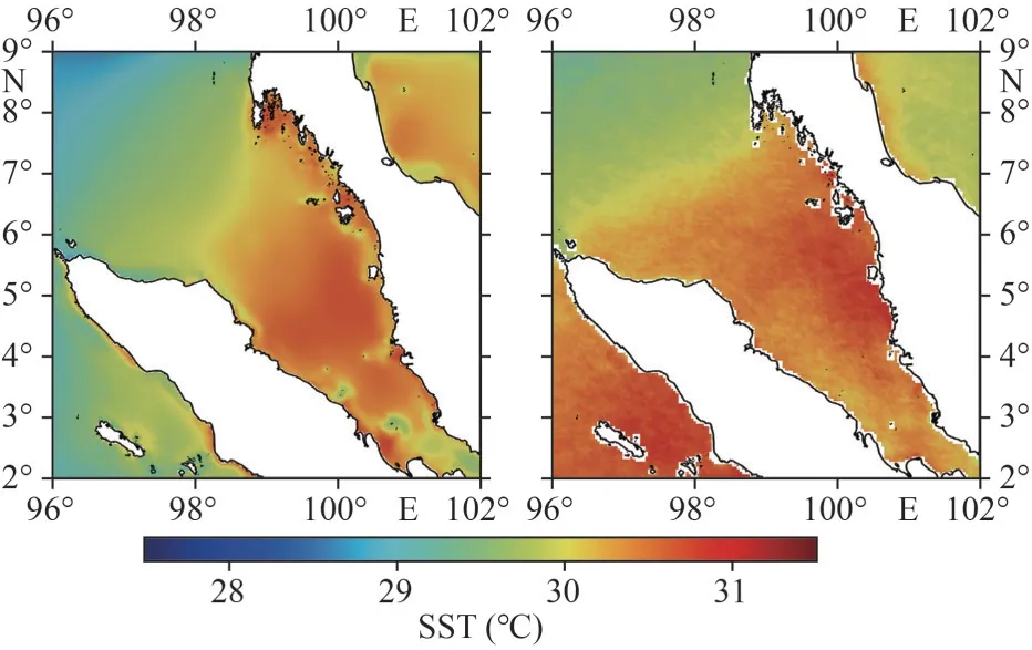
Fig.2 Sea surface temperature (°C) validation during annual climatology (2002-2012) using data from ROMS (left) and AVHRR (right)

Fig.3 Temperature pattern between model (ROMS) and satellite observations (AVHRR) using the monthly average dataset from the year 2002 to 2012
It is important to note that the comparison of ROMS with AVHRR or Argo can have a bias due to several possible resources.From the perspective of ROMS, the combination of strong monsoon wind flow direction with bathymetry and topography at different entrance points, the model output can deviate from observation.Furthermore, the strong influence of winds can change the vertical turbulent and vertical advection/convection in the upper layer explaining why temperature is slightly underestimated.Another reason could arise from the changes in the vertical resolution at different locations due to the vertical configuration of the model (Lonin et al., 2010).For AVHRR, because it is satellite-based, AVHRR’s ability to accurately observe shallow water areas like Malacca Strait is limited.Finally, yet importantly, for Argo, who employed a profiling float to conduct observations,there were challenges in covering the data resolution.Generally, the constraints must be taken into consideration during the evaluation process.

Fig.4 Monthly mean climatology of the temperaturedepth profile from ROMS (blue line) and Argo float(black line) data in the northern MS region
3.2 Model-derived SST
The monthly analysis of 11 years of climatology data (2002-2012) in Fig.5 shows the SST distribution from January to December.In general,each month shows a different temperature gradient between the Malacca Strait and southern Andaman Sea areas (5°N-8°N, 96°E-99°E).For further discussion, the area of Malacca Strait was divided into three regions which are northern MS (6°N-7.9°N), middle MS (4°N-5.9°N), and southern MS(2°N-3.9°N) (Fig.1).Generally, the temperature was recorded with cooler water during the northeast monsoon (December, January, and February) in a range of 27-29.5 °C.Meanwhile, during the first intermonsoon in March, April, and May, the temperatures ranged 28-30 °C.In the southwest monsoon (June,July, and August) and second inter-monsoon(September, October, and November) the temperatures ranged 29-31 °C and 30-31 °C, respectively.
Throughout the northeast monsoon, the temperature in the east of Sumatra varies from the temperature off the west coast of Peninsula Malaysia and south of Thailand.In February, the temperature in the east of Sumatra is cooler than on the other side, with a temperature of ~27.5 °C in Sumatra while on the other side in the range of 28.5-29.5 °C due to the wind blowing from the north and northeast to the south-west, which brings warm water from east Sumatra towards the west of Peninsular Malaysia(Rizal et al., 2012).During February, a group of warm water can be seen collecting near the west coast of Thailand, surrounded by lower temperatures.It is formed when cold water from the east coast of Sumatra flows into the southern Andaman Sea and collides with warm water from the west coast of Peninsular Malaysia.The convergence between these two different water masses is seen in the middle of the area, but it started to disappear in March and completely disappear in April due to the retraction of the current.
The temperatures in April slightly increased before the warmer water from the middle of Malacca Strait was pushed towards the northern Malacca Strait and the southern Andaman Sea from May until August.This condition could arise because of the high levels of solar radiation in this area.According to Irwan et al.(2015), Bayan Lepas(Penang), which is one of the regions closest to the middle Malacca Strait, has a high value of solar radiation.In this period, three different SST values(29, 30, and 31 °C) were observed from the middle of Malacca Strait towards the southern Andaman Sea in the north and the middle of Malacca Strait towards the southern Malacca Strait.This could be owing to the Indian Ocean having colder temperatures, which are caused by the region having considerable precipitation brought by the prevailing winds.As a result, the strait is warmer and the Andaman Sea has a cooler temperature (Isa et al., 2020).
During May, it has slightly cooler temperatures than the others ranging 28.5-29.5 °C, and August has warmer temperatures, ranging 28.5-31 °C.From June to August, warmer water in the middle of Malacca Strait exacerbated the temperature gradient to the southern part of Malacca Strait.The middle of the Malacca Strait is warmer than other areas due to its narrow feature and being blocked by the lands.It caused heat exchange between sea and air to be slower than in the northern part of the Malacca Strait where it is more exposed to the open ocean.In such a situation, the probability of the occurrence of a thermal front in this area is high (Ilhamsyah et al.,2018).
During September, October, and November, the water in the southern region experienced warmer temperatures.In December, new SST contours of 28.5-30 °C were observed along between the southern Andaman Sea and Malacca Strait, replacing the previous month’s SST contour of 31 °C.Overall, in this study area, the temperature increases gradually as water enters the shallow area.This was also the case when the shallow part of Malacca Strait was found to have a higher temperature than the deeper areas of the southern Andaman Sea.
3.3 SST front detection using SIED during monsoon season
Table 1 shows the summary of the horizontal distribution of temperatures at 10-, 25-, 50-, and 75-m depths in February, May, August, and November from 2002 to 2012.Based on the results, the occurrence of thermal fronts varied for those months.Most of the thermal fronts occur during February and May in various depths.This could be due to the northeast monsoon transitioning to the first intermonsoon, which is quite noticeable because it transitions from cool to warmer temperatures, as opposed to the southwest monsoon transitioning to the second inter-monsoon, which is less noticeable due to similar warmer temperatures during this period.In addition, with the condition between the southern Andaman Sea and Malacca Strait, which receives water from the open ocean such as the Andaman Sea and shallower Malacca Strait, a significant temperature difference will inevitably occur, resulting in the formation of thermal fronts.
From Table 1, in February, most of the front occur in a depth of 10 m in the years 2003, 2004,2006, and 2007, the rest of the depth, 25 m (2002 and 2004), 50 m (2002 and 2005), and 75 m (2005 and 2007).For May, 50 m has most of the thermal front which is 2002, 2003, 2004, 2005, 2007, and 2009, followed by 10 m (2002 and 2003), 25 m(2003 and 2007), and the last one 75 m (2002 and 2003).Surprisingly, the thermal front during August and November for all years is untraceable aside from the years 2007 (50 m), 2010 (75 m), and 2011(10 m).The thermal front in the years 2007 and 2010 appear in November while the thermal front during the year 2011 occurred in August.Generally,most of the thermal front occurs in the first two seasons (February and May) compared to the last two seasons (August and November).Based on the result, surprisingly, in the year 2003, the thermal front was present at each depth (10, 25, 50, and 75 m) in May.However, in the year 2010, the thermal front only occurs in the bottom layer(75 m).For further discussion, the normal year which is 2003 (subtopic 3.3.1) was chosen since it had a thermal front presence at each depth, and 2010(subtopic 3.3.2) represents the El-Ni?o year and negative Indian Ocean Dipole (IOD).
3.3.1 Thermal front during the normal year
Figure 6 shows the distribution of SST at 10, 25,50, and 75 m during May 2003.The left figure shows the location of the thermal front at the selected depth and the right panel shows the crosssectional vertical profile for the thermal front from the left panel.The location of the detected thermal front is marked with black lines and labeled with “F”.In addition, the cross-sectional distribution of temperature across the selected front (marked as F1,F2, F3, and F4) was presented.As mentioned above,we used the year 2003 to further discuss the thermal front variability in the study area.Figure 6 showsthe surface thermal front at 10-m depth occurs between northern Malacca Strait and the southern Andaman Sea near Thailand’s coastal water.According to the cross-sectional temperature profile(Fig.6a), the surface warm pool at the northern Malacca Strait and the cooler Andaman’s Sea surface water had caused a significant horizontal temperature gradient, which caused the formation of the frontal zone.

Table 1 The existence of the thermal front based on selected months from 2002 to 2012

Fig.6 The distributions of the thermal front overlay with SST (left) and cross-sectional vertical profile of SST (right) at different depth for year 2003
The thermal front was identified at a depth of 25 m in the southern Andaman Sea area marked as F2.The existence of a thermal front area was discovered when cooler temperatures from the east of the Indian Ocean attempted to infiltrate the warmer southern Andaman Sea.The presence of a thermal front area is less apparent in a crosssectional vertical profile (F2) compared to F1.The thermal front could happen due to the effects of the transition period from northeast monsoon to the first inter-monsoon between the southern Andaman Sea and Malacca Strait, which leads to the formation of fronts at the boundary line between two different temperature values and is often associated with mixing (Kumar et al., 2009).
In addition, the thermal front appears at a depth of 50 m in three locations: the southern Andaman Sea, northern Malacca Strait, and middle of Malacca Strait.When warmer seawater from the southern Andaman Sea meets with cooler water from the east of the Indian Ocean, a thermal front would form at the boundary line between the regions.Meanwhile,at F3, the thermal front in the north of the Malacca Strait formed when the warmer seawater surrounds the cooler seawater as an eddy formed in the area.Another front formed in the middle of Malacca Strait when the cooler seawater temperature from the southern Malacca Strait collided with the warmer temperature from the middle of the Malacca Strait, causing the formation of a thermal front in that particular area.This could be due to the area of southern Malacca Strait being comparatively shallow compared with the middle of Malacca Strait.The shallower area experiences warmer temperatures compared to the deeper areas.The convergence of two different water masses caused the formation of a thermal front in the area.
The southern Andaman Sea has experienced a thermal front appearance at the bottom surface(75 m).The thermal front condition at this depth(F4) shows the same characteristics as F2 because the converging of two masses of water from the open sea and the shallow sea often causes the thermal front occurrence.Subsurface water (24-26 °C) intrudes into the southern Andaman Sea and the thermocline follows the bottom topography and meets the cooler temperature (~23 °C).
3.3.2 Thermal front during the El Ni?o and negative IOD year
Figure 7 shows the distribution of SST at 10 m (a),25 m (b), 50 m (c), and 75 m (d) during November 2010.As shown in Table 1, 2010 was the El Ni?o and negative IOD year, the thermal front occurred at 75-m depth (see black line in Fig.7d) only.There is no thermal front detected in a shallower area than 75 m (Fig.7a-c).Figure 7e shows the cross-section vertical profile for the thermal front denoted as F5 in Fig.7d.In this situation, the thermal front occurs when the cooler water from the southern Andaman Sea meets the warmer water from the northern Malacca Strait.
3.4 Relationship between the thermal front and Chl a towards productivity
This subtopic will discuss the relationship of Chlawith the thermal front.There is some limitation when addressing Chlain this study.Chlorophyll-aproduction in marine environments is indeed complex and is influenced by several factors including physical, chemical, and biological.This study focuses on the physical distribution of Chlain an area where thermal fronts are formed and not involving any chemical or biological experiments.Based on Fig.8, the Chl-agradient occurs in the same area as the thermal front.The Chl-aconcentration shows the highest on the side of Malacca Strait rather than the southern Andaman Strait.Based on the spatial correlation between SST and Chlapresented in Fig.9, a 0.5 positive correlation at a 95% confidence level with SST of ~31 °C and Chl-avalue ~0.5 mg/m3was observed at the location of the thermal front.Other than May 2003, thermal front and spatial correlation during Feb.2004, Feb.2006, and Feb.2007 were calculated and presented in Fig.10.The location of the front can be seen through the black line in the ocean (left side of Fig.10) while the spatial correlation for the front can be seen in the black box in the ocean (right side of Fig.10).During Feb.2004 (Fig.10a), the spatial correlation of the front has a dominant negative spatial correlation of approximately -1 at 95% confidence level.For the Feb.2006 and Feb.2007, dominant positive spatial correlation approximately 1 at 95% confidence level was observed.According to the results, high concentration of Chladoes not guarantee the presence of a thermal front, but when a thermal front appears, the concentration of chlorophyll in the area is high (Fig.9).

Fig.7 The distributions of the thermal front overlay with SST during November 2010

Fig.8 Distribution of (left side) and (right side) during May 2003 on surface water

Fig.9 Spatial correlation between SST and Chl a during May 2003 on surface water
This research found that the thermal front on the side of Malacca Strait has is higher compared with the southern Andaman Sea.To support the findings,this research tries to discover the thermocline layer.The thermocline layer has taken part in vertical mixing, combined with frontal circulation could bring nutrient-rich subsurface water into the surface euphotic zone, thus making the frontal region a conspicuous place for primary production.In May 2003 (the same data were used in Fig.6a), two points were chosen (based on the thermal front location of F1) to represent the southern Andaman Sea (located northern the thermal front area) and the Malacca Strait (located at the southern of the thermal front area) for investigation of the thermocline layer.The detail of the points is shown in Table 2.Analyses of the thermocline profile and thermocline layer are shown in Fig.11 and Table 3.The thermocline location was determined based on ΔT/Δz≥0.1 °C/m (Irmasyithah et al., 2019).The distribution of the thermocline profile at selected points depicted temperature changes according to depth.The thermocline profile was divided according to the mixed layer, thermocline layer, and deep layer.In May 2003, the result shows the thermocline layer varied between those two areas, Malacca Strait and the Andaman Sea.The thermocline layer was at a depth of 10-70 m for Malacca Strait and 80-120 m for the southern Andaman Sea.According to Irmasyithah et al.(2019), the thermocline layers in the Andaman Sea are less than 200 m, which supported the result of this research.The thermocline layer in the Malacca Strait had a temperature ranging 21-28 °C, whereas the southern Andaman Sea ranges 19.5-25 °C.The thermocline gradient in Malacca Strait was 0.12, and in the southern Andaman Sea, it was 0.14.
4 DISCUSSION
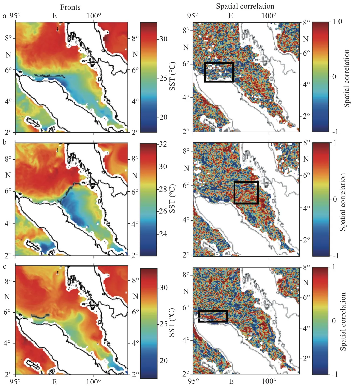
Fig.10 Fronts and spatial correlation (SST vs.Chl a) during Feb.2004 (a), Feb.2006 (b), and Feb.2007 (c)

Table 2 The detail of the two selected point
The thermal front in the southern Andaman Sea and Malacca Strait was investigated by using 11-year ROMS-derived SST outputs.Selected monthly data were used to identify the SST front for each monsoon season.The climatological dataset was not used since it has an inherent flaw in recognizing fronts due to the smoothing effects of temperature profiles including incursion, interleaving, and inversion, weakening frontal intensity, and blurring a clear frontal zone (Park and Chu, 2006).The results show that the thermal front between the southern Andaman Sea and Malacca Strait has a similar demarcated area as found by Ilhamsyah et al.(2018)who reported thermal front occurrence on the northern coast of Aceh from March to May by using model outputs of SST and baroclinic circulation.However,in their study, the thermal front was identified directly from the model outputs without using an algorithm to calculate the temperature gradient to prove the appearance of the thermal front.Furthermore, the use of the model by Ilhamsyah et al.(2018) covers a horizontal resolution of about 1/12° compared to the ROMS model in this study which is 1/30°.
According to Table 1, thermal fronts mostly occurred during February (representing the northeast monsoon) and May (representing the first intermonsoon) and less in August (representing the southwest monsoon) and November (representing the second inter-monsoon).This may be related to the changes in physical properties and current circulation due to the monsoon.Different directions and intensity of currents circulation and physical properties between the Malacca Strait and southern Andaman Sea during the northeast monsoon and first inter-monsoon converges and caused greater horizontal gradient differences between both areas(Fig.12a, b).Thermal front was formed in this convergence zone.The thermal front is less occurred during the southwest monsoon (Fig.12c) and the second intermonsoon (Fig.12d) because the currents around the Malacca Strait and the Andaman Sea are at the same speed and collide slowly, resulting in weaker gradient differences.

Fig.11 Thermocline profile during May 2003 at Malacca Strait (a) and southern Andaman Sea (b)

Table 3 Thermocline layer for the selected point in Malacca Strait and the southern Andaman Sea in May 2003
The geographical location of the southern Andaman Sea and Malacca Strait, which are influenced by El Ni?o and IOD, would give a significant impact on the thermal front variations.According to Luu et al.(2014), ENSO affects the sea level over the Malaysian coast while IOD modulates sea level anomalies mainly in the Malacca Strait.In the Andaman Sea, these events slowed the growth of coral on the reef as the events modulate the sea level and temperature of the sea(Dunne et al., 2021).In this study, the thermal front occurred at each depth in a normal year (2003).However, during the El Ni?o and negative IOD year(2010), the thermal front occurred only at a depth of 75 m.The negative IOD means wetter in the Indian area and drier in the Peninsula Malaysia area.The absence of thermal front occurrence in the surface area in 2010 could be related to El-Ni?o and negative IOD when Isa et al.(2020) reported that Malacca Strait experienced both El Ni?o and IOD in 2010 when the surface temperature is extremely high.It is when the high temperature at the surface and also in the thermocline area prevents the uplifting of cold water.This indicates that the El Ni?o and negative IOD phenomena will limit the existence of the thermal front and disturb marine products in the area, particularly near the sea surface area.

Fig.12 Seasonal climatology current circulation (m/s) and sea surface temperature (°C) during northeast monsoon (a), first inter-monsoon (b), southwest monsoon (c), and second intermonsoon (d) from 2002 until 2012
Due to the topographical area, the thermal front in the southern Andaman Sea and Malacca Strait region occurs at a shallower depth during the normal year (2003).Because the thermal inertia of a water column on the shelf is linearly proportional to the bottom depth, the sea surface temperature is highly influenced by the bottom depth due to the research location area that was located on the continental shelf.Bottom topography causes SST and climate factors like surface wind, heat flux, and cloud cover to interact (Xie et al., 2002).The Kuroshio front develops when the warm stream meets the considerably colder shelf water whereby the same happens in the southern Andaman Sea and Malacca Strait area when warm water from Malacca Strait meets cooler water from the southern Andaman Sea.Without the presence of phenomena such as El Ni?o, the thermal front remained untouched,allowing it to be present at every layer of depth.
Thermal fronts, as hydrologic structures, have a variety of effects on an organism’s distribution,including taxonomic selection and increased productivity.In other words, fronts have biological and chemical manifestations.Once a property of the front is detected, consequently, another frontal property will be detected accordingly.The simultaneous physical, chemical, and biological manifestations of the same front are considered to be located in the same position, although there is a relatively small difference in distance (Belkin et al.,2009).Although thermal zone exists in relatively small areas in the southern Andaman Sea and Malacca Strait, they play an important role in ecological processes, allowing for high biological production, providing feeding and reproductive habitats for fishes, squids, and birds, acting as retention areas for larvae of benthic species and promoting the establishment of benthic invertebrates that benefit from the organic production in the frontal area (Acha et al., 2004).
In this research, the influence of surface thermal fronts over the surface Chl-aconcentration in the southern Andaman Sea and Malacca Strait at a monthly scale was measured subjectively.According to the findings of this study, more Chlais found in areas with higher temperatures.The presence of the highest Chlaat the high-temperature side of the front location can be attributed to the intensity of the light entering the waters and the nutrient content in the waters.This condition could be caused potentially by freshwater influx from the west coast of Peninsular Malaysia and the East of Sumatra (Thia-Eng et al., 1997; Jaya et al., 1998; Pang and Tkalich,2003; Hii et al., 2006).The center portion of Peninsular Malaysia has several large river systems(Perak, Bernam, Selangor, and Klang rivers).Aside from that, compared to the deep sea like the Andaman Sea, the shallow and narrow Malacca Strait area close to the shore would normally have a higher Chl-aconcentration because nutrients will flow from the land (agricultural activities) to the seawater bringing high nutrient, whereas, the deep ocean has low Chl-aconcentration because it does not receive nutrients directly.Despite this reason, the thermal front area adjacent to the Malacca Strait has higher productivity than the thermal front area adjacent to the Andaman Sea.Chlorophyllais used as information to assess the fish resources because there is a relationship between primary productivity and fisheries resources.Thus, it can be said that the area with high Chl-aconcentration has high fish assemblages (Mahabror et al., 2017).This is because Chlahas a high nutrient content, which can suggest a higher productivity area for marine resources.Therefore, the Chl-adata from satellite MODIS Aqua will be used to examine the link between SST and Chla.
In vertically homogenous water, there is good nutrient availability, while stratified water receives enough light levels.This is why photosynthetic activity in the shelf is highly dependent on the stability of the water column.A superficial thermal front is an indicator of the confluence of stratified and mixed water (Rivas, 2006).Besides that, Irmasyithah et al.(2019) mentioned that thermocline layers play a significant role in thermocline flows, upwelling,and fish migration.The thermocline limits will shift as a result of this factor, as will the fishing area and Chl-acontent (Saji et al., 1999; Kunarso et al.,2012).In other words, thermocline layers have an impact on nutrient distribution.As a result, this theory has been verified in the area between the southern Andaman Sea and Malacca Strait by analyzing the thermocline profile to investigate the water column in the thermal front area.From the analysis, the thermocline layer at the Malacca Strait is located in a shallow area compared to the southern Andaman Sea (Fig.11).The shallower the location of the thermal front, the easier it is for water to bring Chlato the surface.This statement is supported by Sprintall et al.(2003), the shallow thermocline layer supported aquatic productivity which is during a vertical process, nutrients in the shallow thermocline layer would more easily reach the surface layer than the deeper thermocline layer.Interestingly, Fig.8 shows that the Chlafrom the satellite in this area was also high which means the presence of nutrients will further increase Chl-aconcentration.This situation demonstrates how the Malacca Strait region outperforms the southern Andaman Sea in terms of productivity.In the Malacca Strait, the presence of anticyclonic eddy during the occurrence of the thermal front in May 2003 limits and spread the Chlaspreading over the entire Malacca Strait (Fig.13).Eddies play an important role in modulating the physical, chemical,and biological properties of the ocean (Devresse et al.,2022).As a result, the presence of eddy and front at the same time helps in the distribution of Chla.
Vertical mixing process as well as stratification also play important roles in regulating Chlawithin the water column.The thermocline in shallow areas like Malacca Strait can easily deliver nutrients to reach surface water compared to the thermocline in the deep area.Furthermore, the thermocline in the shallow area also has high phytoplankton because the area receives enough light for the photosynthesis process while phytoplankton was limited at the thermoclines in the deep area (Cantin et al., 2011;Jamshidi and Bin Abu Bakar, 2011).According to that reason, the shallower thermocline layer benefited aquatic productivity.Increasing ocean water stratification will only result in nutritional deficiency, reduced biomass, and selection for smaller cells (Morán et al., 2010; Flombaum et al.,2013; Kang et al., 2021).In general, during May 2003, it can be concluded that the location of the thermal front on the side of the Malacca Strait area consists of high productivity compared to the southern Andaman Sea area based on the thermal front area and Chl-adistribution.
5 CONCLUSION
This thermal front detection using the SIED algorithm in this study has provided new information on the spatial and seasonal distribution of ocean fronts between the southern Andaman Sea and Malacca Strait.It is apparent that where the area between the southern Andaman Sea and Malacca Strait bathymetry influences the current, which is also exhibited in the patterns of front observations.While El-Ni?o and IOD have an effect on the distribution of the thermal front, as seen in this study, the event that causes the thermal front only occurs at the bottom depth.The presence of a thermal front throughout the water column gives an important impact on biological productivity.In this study, the approach of using Chl-adata and analyzing the vertical profile to see the influence of thermal fronts on the abundance of phytoplankton is one of the good elements.Throughout the analysis, the Malacca Strait is unique and privileged which is surrounded by Peninsula Malaysia and Sumatra, as well as receiving freshwater from nearby rivers, making it rich in biological resources compared to the southern Andaman Sea.Further research is needed to elucidate the generalization of this relationship, for example, to estimate the size and depth of topographic features that can influence the generation of the thermal front.
In conclusion, thermal fronts in the southern Andaman Sea and Malacca Strait are easy to identify and locate.Although the location of thermal fronts is within the well-defined areas, it is still difficult to associate them with clearly defined high-productivity areas.However, the results of this study could serve as a starting point for future research on higher productivity, and it is recommended that the location of the thermal front as fishing grounds be further explored to avoid overfishing.To determine the location of pelagic fish (commonly inhabit in the pelagic zone of the ocean), the thermal front needed to be identified.The department of fisheries can share this knowledge with fishermen to help them in their daily lives.By providing this information, the fisherman can determine the best time to go and fish at the fishing grounds for a higher catch rate.Lastly, it should be noted that this study does not examine the factors that contribute to the occurrence of the front,hence, it is recommended that future research be conducted to identify the factors like eddies that may contribute to the occurrence of the front in between the southern Andaman Sea and Malacca Strait.
6 DATA AVAILABILITY STATEMENT
In this study, the required data can be freely downloaded from several websites.Reanalysis data for current, sea surface temperature, and sea surface salinity are available on the HyCOM website at https://www.hycom.org/data/glbu0pt08/expt-19pt1.Bathymetry data can be obtained from the GEBCO website at https://www.gebco.net/data_and_products/gridded_bathymetry_data/.Sea surface temperature data from satellite sources can be found on the AVHRR website located at https://www.ncei.noaa.gov/access/metadata/landing-page/bin/iso?id=gov.noaa.nodc: AVHRR_Pathfinder-NCEI-L3C-v5.3.Temperature by water depth data from Argo Float can be accessed through http://sio-argo.ucsd.edu/RG_Climatology.html.Additionally, tidal, wind, and chlorophyll-adata are available at the following websites: https://www.tpxo.net/global for tidal data,https://www.ecmwf.int/en/forecasts/dataset/ecmwfreanalysis-v5 for wind data, and https://oceancolor.gsfc.nasa.gov/l3/ for chlorophyll-adata.Lastly, for atmospheric data can be access at ERA5 website which is available at https://www.ecmwf.int/en/forecasts/dataset/ecmwf-reanalysis-v5.
 Journal of Oceanology and Limnology2024年1期
- Journal of Oceanology and Limnology的其它文章
- Contrasts of bimodal tropical instability waves (TIWs)-induced wind stress perturbations in the Pacific Ocean among observations, ocean models, and coupled climate models*
- Variability of the Pacific subtropical cells under global warming in CMIP6 models*
- Magmatic-tectonic response of the South China Craton to the Paleo-Pacific subduction during the Triassic: a new viewpoint based on Well NK-1*
- An improved positioning model of deep-seafloor datum point at large incidence angle*
- Microplastics in sediment of the Three Gorges Reservoir:abundance and characteristics under different environmental conditions*
- Spatial patterns of zooplankton abundance, biovolume, and size structure in response to environmental variables: a case study in the Yellow Sea and East China Sea*