Contrasts of bimodal tropical instability waves (TIWs)-induced wind stress perturbations in the Pacific Ocean among observations, ocean models, and coupled climate models*

Kai MA, Chuanyu LIU, Junli XU, Fan WANG

1 School of Mathematics and Physics, Research Institute for Mathematics and Interdisciplinary Sciences, Qingdao University of Science and Technology, Qingdao 266100, China

2 Key Laboratory of Ocean Circulation and Waves, Institute of Oceanology, Chinese Academy of Sciences, Qingdao 266071,China

3 Pilot National Laboratory for Marine Science and Technology (Qingdao), Qingdao 266237, China

Abstract The coupling between wind stress perturbations and sea surface temperature (SST)perturbations induced by tropical instability waves (TIWs) in the Pacific Ocean has been revealed previously and proven crucial to both the atmosphere and ocean.However, an overlooked fact by previous studies is that the loosely defined “TIWs” actually consist of two modes, including the Yanai wave-based TIW on the equator (hereafter eTIW) and the Rossby wave-based TIW off the equator (hereafter vTIW).Hence, the individual feedbacks of the wind stress to the bimodal TIWs remain unexplored.In this study,individual coupling relationships are established for both eTIW and vTIW, including the relationship between the TIW-induced SST perturbations and two components of wind stress perturbations, and the relationship between the TIW-induced wind stress perturbation divergence (curl) and the downwind(crosswind) TIW-induced SST gradients.Results show that, due to different distributions of eTIW and vTIW, the coupling strength induced by the eTIW is stronger on the equator, and that by the vTIW is stronger off the equator.The results of any of eTIW and vTIW are higher than those of the loosely defined TIWs.We further investigated how well the coupling relationships remained in several widely recognized oceanic general circulation models and fully coupled climate models.However, the coupling relationships cannot be well represented in most numerical models.Finally, we confirmed that higher resolution usually corresponds to more accurate simulation.Therefore, the coupling models established in this study are complementary to previous research and can be used to refine the oceanic and coupled climate models.

Keyword: bimodal tropical instability waves; mesoscale air-sea interaction; coupled models; Yanai wave

1 INTRODUCTION

Satellite observations show that strong air-sea interactions occur in the mesoscale vortexes of the Kuroshio and Gulf Stream extensions, the Antarctic Circumpolar Current and the sides of the Pacific Cold Tongue (Chelton et al., 2004; Xie, 2004; Small et al., 2008; Bryan et al., 2010; Kelly et al., 2010;Putrasahan et al., 2013; Ma et al., 2015).Tropical instability waves (TIWs) in the Pacific equatorial cold tongue are representative mesoscale westward propagating equatorial waves, which have been found in sea surface temperature (SST), sea level height,ocean salinity, and sea surface chlorophyll concentration(Legeckis, 1977; Chavez et al., 1999; Chelton et al.,2000; Menkes et al., 2002).TIWs occur approximately from July to the end of January of the next year.The length of TIWs is about 600-1 500 km, the period is 15-40 d, and the westward propagation speed is 30-80 m/s (Chelton et al., 2000; Jin et al., 2015).

The air-sea interaction induced by TIWs has been long studied.Satellite observations show an obvious relationship between TIW-induced wind stress (τTIW)and SST (SSTTIW), Xie et al.(1998) found that theτTIWnear the cold tongue is in phase with the SSTTIW,and pointed out that TIWs can affect wind stress and atmospheric boundary layer.Satellite observations revealed that these interactions are not only manifested by a correlation between the SSTTIWand the magnitude of theτTIW, but also by a significant linear relationship between theτTIWdivergence (curl) and downwind(crosswind) SSTTIWgradient (Chelton et al., 2001,2004, 2007; Thum et al., 2002).

In addition, it is further found that when introducing an empirical relationship betweenτTIWand SSTTIWbased on satellite observations into numerical models(Pezzi et al., 2004; Zhang and Busalacchi, 2009), theτTIWcan dampen the strength of SSTTIW(Small et al.,2008), modulate the low-frequency variability of the ocean, and influence the mean state of the ocean(Pezzi et al., 2004; Zhang and Busalacchi, 2008; Zhang,2014, 2016).Recently, Wei et al.(2018, 2019) used satellite observations to develop sophisticated empirical models betweenτTIWand SSTTIW, and constructed the empirical model from the relationship between the derivative field ofτTIWand SSTTIWgradient.By comparing two parallel experiments with and without theτTIW, they demonstrated thatτTIWhas a significant impact on the equatorial Pacific heat budget, causing a long-term mean SST change of 0.2 °C.This suggests that the air-sea interaction caused by TIW does play an important role in the ocean.

Therefore, it becomes obvious that this air-sea interaction needs to be adequately considered in both the ocean general circulation models and the fully coupled climate models.However, since the forcing fields used in oceanic models are generally derived independently from other databases, the scale of wind fields cannot fully match the oceanic mesoscale.Moreover, in coupled climate models, their simulations of the ocean are often subject to errors due to coarse spatial resolutions and difficulties in accurate parameterization of relevant processes in the ocean or atmospheric boundary layer (Spall, 2007; Song et al., 2009; Chelton and Xie, 2010).Thus, numerical models often failed to represent air-sea interaction adequately (Maloney and Chelton, 2006; Bryan et al., 2010), thus it is always difficult to interpret the observations for accurate forecasts.Therefore, it is necessary to specifically evaluate the performances of current ocean general circulation models and coupled climate models in representing the air-sea interaction induced by bimodal TIWs in order to facilitate model improvements.

Meanwhile, several studies have revealed that there are two modes of TIWs in the eastern equatorial Pacific, rather than the loosely defined one kind of TIW (Halpern et al., 1988; Flament et al., 1996; Lyman et al., 2007; Liu et al., 2019): one is the equatorial mode (eTIW) by Liu et al.(2019)and the other is the Rossby mode TIW.The eTIW is centered at the equator, with a period of about 17 d.Structurally similar to Yanai waves, the eTIWassociated temperature anomalies show a meridional asymmetric structure (Lyman et al., 2007), and its velocity shows a northeast-southwest flow pattern.The Rossby wave mode TIW is the one in traditional concept and research, which is centered at 4°N-5°N with a period of about 33 d.In addition, it is similar in nature to unstable Rossby waves, showing similar maxima center of temperature on both sides of the equator (a little larger in north of the equator), and almost no meridional velocity at the equator.This mode is usually strong so it manifests itself as a vortex (Flament et al., 1996), hence the name vortex mode TIW (vTIW).In general, the two modes of TIWs were revealed for having different properties,but less is known about eTIW.Liu et al.(2019)focused on the horizontal flow structure of eTIW,the location of its occurrence, and its effect on equatorial mixing, demonstrating that eTIW may have important implications for regulating vertical mixing/heat transport in the global ocean.

On the one hand, the centers of eTIW and vTIW are located at the equator and 4°N, respectively.On the other hand, the wind stress at the equator differs from that in the north, which gradually tilts northward from the equator to the north.Therefore,it is speculated that the air-sea interactions induced by eTIWs and vTIWs may differ.However,previous studies on the air-sea interaction induced by TIWs did not consider these contrasts nor explore whether differences exist between the twomodes-induced coupling; instead, they usually loosely considered “TIW” as a one-mode phenomenon.

Therefore, TIW-induced air-sea interactions are critical to both the ocean and atmosphere, previous studies did not mention that TIWs has two modes.We focused on the neglected individual air-sea interactions induced by bimodal TIWs.The major aim of the present work was to focus on the bimodal TIWs separately to investigate whether and to what extent the two modes of TIWs can lead to the previously recognized air-sea interactions.In addition,we will also investigate how the advanced ocean general circulation models and coupled climate models represent such interactions.

In this manuscript, Section 2 introduces the data and main methods used in this paper.In Section 3,the bimodal TIW-induced air-sea interactions are studied based on satellite observations, and the relationship betweenτTIWand SSTTIWinduced by bimodal TIWs was quantified to establish the coupling models.In Sections 4 and 5, interactions between bimodalτTIWand SSTTIWwere examined in several widely accepted ocean general circulation models and fully coupled climate models.Section 6 presents the main results with the discussions and conclusions.

2 DATA AND METHOD

2.1 Data

2.1.1 Satellite observation

This paper uses the optimally interpolated (OI)0.25°×0.25° daily SST reanalysis data (NOAA OISST V2.0) as the observations of SST.Several sources including AVHRR satellite daytime and nighttime observations, buoys-based and ship-based observations are merged during interpolation, using pre-computed error characteristics as weights.More details can be found in Reynolds et al.(2007).We note that since the OISST product is obtained with Optimum Interpolation v2, which has smoothed the original satellite-based observational data to some extent, as a result, the SST perturbation could be a little bit smaller than the real.

The wind field data used in this study is the Advanced SCAT thermometer (ASCAT) from the European Meteorological Satellite Organization(EUMETSAT).ASCAT data are produced by Remote Sensing Systems and sponsored by the NASA Ocean Vector Winds Science Team, whose main mission is to provide global ocean surface wind vector business products (Figa-Saldana et al., 2002; Bentamy et al.,2008; Verspeek and Portabella, 2010).Data are available at www.remss.com.This study used the product of 0.25°×0.25° in resolution (Ricciardulli and Wentz, 2016).

The high-resolution and dense sampling of contemporaneous satellite-based ASCAT and OISST data provides opportunities for the study of air-sea interactions caused by bimodal TIWs in the tropical Pacific.The time range of satellite observations analyzed was set from January 1, 2008 to December 31, 2019, 4 383 d in total.

2.1.2 Oceanic general circulation model

In this study, we choose two widely accepted oceanic general circulation models to investigate their capabilities in incorporating the bimodal TIWinduced air-sea interactions.

One model is the HYbrid Coordinate Ocean Model (HYCOM; Bleck, 2002; Halliwell, 2004),which is a data-assimilative hybrid isopycnal-sigmapressure (generalized) coordinate ocean model that is widely used in research (Chassignet et al., 2003,2006).Its assimilation uses the NRL Coupled Ocean Data Assimilation (NCODA) scheme.This model has a high resolution of 0.08°×0.08°, which facilitated the establishment of coupling relationships.The temperature data of the first layer of the model was considered as the SST.The HYCOM-employed wind stress data were hourly NCEP CFSR in resolution of 0.312 5°×0.312 5° and were interpolated into the HYCOM temporal (daily) and spatial grids (0.08°×0.08°) for ease analysis.More details can be found in Cummings and Smedstad (2013).

The other model is the second phase of “The Estimating the Circulation and Climate of the Ocean”(ECCO2).ECCO2 data syntheses were obtained by least squares fit of a global full-depth-ocean and seaice configuration of the Massachusetts Institute of Technology general circulation model (MITgcm;Marshall et al., 1997) to the available satellite and in situ data, the time span was from 1992 to the present.The assimilation method used for ECCO2 was the 4D-VAR based on Green’s function(Menemenlis et al., 2005), i.e., by making optimal adjustment of model parameters, initial conditions,and boundary conditions (atmospheric forcing fields)through a series of sensitivity numerical simulations and minimization of model/observation misfit.The data used to constrain the model included sea surface height, ocean bottom pressure, surface wind stress,satellite based SST products, sea ice concentration and velocity data, and temperature and salinity profiles.The SST and wind stress field in resolution of 0.25°×0.25° were used in this study.

2.1.3 Fully coupled climate model

The Coupled Model Intercomparison Project (CMIP)provides a unique platform for climate science research by coordinating the simulations from multiple comprehensive coupled global climate models developed by different research institutions around the world.As needed, we selected five models with historical data in raw grid format and with daily SST/taux/tauy: CESM2-FV2, CESM2-WACCM,CESM2-WACCM-FV2 from the National Center for Atmospheric Research (NCAR), and MPI-ESM1-2-HR and MPI-ESM-1-2-HAM from the Max Planck Institute (MPI).The first three of these models are based on the same ocean or atmospheric model thus can be controlled for only differing resolutions, allowing them to be used to investigate the performance of the model in relation to resolution.The last two models from MPI have regular grids for ease of handling,and they are widely recognized and representative.

The CESM2-FV2 climate model, released in 2019, includes the following components: for the atmosphere, it adopts the CAM6 model (1.9°×2.5°finite volume grid; 144×96 longitude/latitude grids;32 levels; top level 2.25 mb); for the ocean, it adopts the POP2 model (320×384 longitude/latitude grids;60 levels; top grid cell 0-10 m).The coupled model was run by NCAR (Danabasoglu, 2019a).

The CESM2-WACCM climate model includes the following components: for the atmosphere, it adopts the WACCM6 model (0.9°×1.25° finite volume grid; 288×192 longitude/latitude grids; 70 levels;top level 4.5e-06 mb); the atmospheric model has higher horizontal and vertical resolutions than CESM2-FV2.For the ocean, it adopts the same POP2 model as CESM2-FV2 with the same resolution (320×384 longitude/latitude grids; 60 levels;top grid cell 0-10 m).The model was also run by NCAR (Danabasoglu, 2019b).

The CESM2-WACCM-FV2 climate model, released in 2019 (Danabasoglu, 2020); for the atmosphere, it adopts the WACCM6 model (1.9°×2.5° finite volume grid; 144×96 longitude/latitude; 70 levels; top level 4.5e-06 mb); the same atmosphere model with CESM2-WACCM, but with lower horizontal and vertical resolutions.For the ocean, it is the same as CESM2-FV2 and CESM2-WACCM.The CESM2-WACCM-FV2 model is based on CESM2-WACCM but several WACCM-specific adjustments were made for model consistency at FV2 resolution (Keeble et al.2021).Both wind stress and SST data in the above models are interpolated to 1.125 0°×0.267 1°longitude/latitude grids.

Both wind stress and SST outputs of the above models are interpolated to 1.125 0°×0.267 1° longitude/latitude grids.

The other two coupled climate models are developed by MPI for Meteorology in Germany.They are global coupled atmosphere-land-ocean-sea ice biogeochemistry models (MPI-ESM).The MPIESM1-2-HR climate model, released in 2017(Niemeier et al., 2019), includes the following components: for the atmosphere, it adopts the ECHAM6.3 model (spectral T127; 384×192 longitude/latitude; 95 levels; top level 0.01 hPa).For the ocean, it adopts the MPIOM1.63 model (tripolar TP04, approximately 0.4 °C; 802×404 longitude/latitude grids; 40 levels; top grid cell 0-12 m).The MPI-ESM-1-2-HAM climate model, released in 2017 (Neubauer et al., 2019), includes the following components: for the atmosphere, it adopts the ECHAM6.3 model (spectral T63; 192×96 longitude/latitude; 47 levels; top level 0.01 hPa), the atmospheric model has lower horizontal and vertical resolutions than MPI-ESM1-2-HR.For the ocean, it adopts the MPIOM1.63 model (bipolar GR1.5, approximately 1.5 °C; 256×220 longitude/latitude grids; 40 levels;top grid cell 0-12 m) (Neubauer et al., 2019), the ocean model also has lower horizontal and vertical resolutions than MPI-ESM1-2-HR.For these two models, we re-grid the SST and wind stress data into 1.0°×0.6° longitude/latitude grids.

2.2 Method

2.2.1 Calculation of bimodal TIW-induced perturbations

To reveal the bimodal TIW-induced perturbations,filters will be applied to the data.The periods of eTIW and vTIW are about 17 d and 33 d, respectively.In addition, the wavelengths are 600-1 500 km in range at the equator (Lyman et al., 2007; Liu et al.,2019).Therefore, spatial scales of less than 500 km or more than 1 200 km, and temporal scales of less than 12 d or more than 45 d were removed by filtering, thus to highlight the TIWs-scale features and remove longer-term modes, such as Pacific Decadal Variability (Small et al., 2008).

In this study, we used Lanczos filter (Lanczos,1950) to filter the TIWs signal.Following Liu et al.(2019) and Wu and Bowman (2007), both temporal and spatial filtering were performed.First, 12-24 d and 24-45 d band-pass filtering were used to separate eTIW and vTIW on the temporal scale, respectively(Liu et al., 2019).Second, a 5°-12° zonal band-pass filtering was conducted to finally determine the eTIW- and vTIW-induced perturbations (Wu and Bowman, 2007).This filtering approach is also an important point that distinguishes this study from previous ones.After double filtering SSTeTIWand SSTvTIW, the (τx,τy)eTIWand (τx,τy)vTIWwere obtained,which denote the anomalies induced with TIWs.SSTeTIWand SSTvTIWare collectively referred to as SSTTIW, and (τx,τy)eTIWand (τx,τy)vTIWare collectively referred to as (τx,τy)TIW.

2.2.2 The establishment of the coupling relationships

Wang et al.(2019) and Tang et al.(2021) sorted out the main mechanisms by which mesoscale SST perturbations influence the overlying atmosphere: the downward momentum transport (DMT) mechanism(Wallace et al., 1989) and the pressure adjustment mechanism (Lindzen and Nigam, 1987).First, the DMT mechanism is described by the predecessors:when wind passes from warm to cold water, the responded SST perturbations would enhance the vertical stability of the atmosphere, which could cause a decrease in downward momentum transport.Thus,when the DMT mechanism dominates the atmospheric response, wind speeds decrease over cold SST perturbations, increase over warm water, which results in a dipole-mode wind stress divergence in regions of a single warm (cold) SST anomaly, with divergence (convergence) upstream and convergence(divergence) downstream of the wind (Byrne et al.,2015).From the analysis, we can infer that there is a linear relationship between the downwind SST gradient and the wind stress divergence.However,when the pressure adjustment plays a dominant role,the atmosphere has sufficient time to adjust so that vertical mixing can occur within the atmospheric boundary layer, making heat transported upwards and modifying the temperature.In addition, the surface pressure would also be affected, resulting in a response pattern that closely matches the SST gradient (Chen et al., 2017).As a result, wind stress divergence and sea surface pressure (SLP) perturbations are distributed directly above the centers of SST perturbations, showing monopole response patterns(Frenger et al., 2013).Therefore, there is a linear relationship between the wind stress divergence and SST perturbations.

According to the dipole patterns of wind stress divergence in Wei et al.(2018), DMT mechanism plays a dominant role in the eastern Pacific.There are at least two methods to establish the relationship betweenτTIWand SSTTIW.One is the method proposed by Pezzi et al.(2004) and Wei et al.(2018), who explored the regression relationships between two components of perturbed wind stress and SST.The second method is based on DMT mechanism (Wallace et al., 1989) and previous studies (Chelton et al., 2004; Wei et al., 2018, 2019;Tang et al., 2019), which explores the relationship between the perturbed wind stress divergence (curl)and downwind (crosswind) SST gradients.The calculation formulas of wind stress divergence (curl)and SST gradient are as follows:

According to Wei et al.(2018), this study established models betweenτTIWand SSTTIWfrom the following two methods: the first model is (τx,τy)TIW=(ax,ay)SSTTIW; the second model is about(divτ)TIW,(curlτ)TIW, and ?SSTTIWinduced by bimodal TIWs:(divτ)TIW=a1×(s·?SSTTIW) and (curlτ)TIW=a2×(n·?SSTTIW).For these two methods, we first need to confirm the correlations between the variables.For the variables with significant correlations, we can establish corresponding regression models, with the regression coefficients of the models being regarded as the coupling strength betweenτTIWand SSTTIW.

2.2.3 Composite analysis

To explore the relationships between SSTTIWandτTIWmore clearly, and try to avoid the interference of irrelevant signals, to depict the spatial relationship between them, we selected some of the data according to specific features as the representatives of TIW-induced perturbations to highlight the desired information.Composite analysis can just meet this purpose, which means to combine samples with some identical characteristics and then get the overall characteristics by analyzing the sample combination.

In this study, each daily data has a matrix ofn×m.Taking SST data as an example: first, we selected a standard point with a highly active TIW, and then following the SST time series of that point, the datei(i=1, 2, …,k) could be found where the SST peak is located, from which then×mmatrix of SST of this date was taken as a sampleX(i)(i=1, 2, …,k).Using these samples as a composite, the composite data matrix was calculated using Eq.2, which can represent this class of samples and be used to characterize the SST perturbations in space.In this way, we calculated the composite matrix of SSTTIWandτTIW,which shows the spatial relationship more clearly and improves the computational efficiency.

2.3 The study area

Fig.1 The mean SST (colors, unit: °C) and wind stresses(vectors, unit: N/m2) averaged over September 1-7 in 2008 in the eastern tropical Pacific (180°-80°W,10°S-10°N)

The eTIW- and vTIW-induced air-sea interactions are considered in the domain 10°S-10°N, 180°-80°W(Fig.1), where very active TIWs were observed(Fig.2).In this region, the “cold tongue” extends westward from the coast of South America to the central equatorial Pacific with seasonal and interannual characteristics (Deser and Wallace, 1990; Mitchell and Wallace, 1992), favoring the generation of the TIWs.In the meanwhile, the southeast-northwest trade winds prevail, providing the background wind filed.However, when the wind passes over the cold tongue, it is decreased significantly to one quarter of its original strength (Chelton et al., 2000).Later, it returns to nearly its original strength when reaching the north of the cold tongue.It is worth noting that in the southern hemisphere west of 160°W, the wind direction has obvious deflection from SE-NW to E-W,which may lead to differences in sea-air interactions at different locations afterward.

3 AIR-SEA COUPLING RELATIONSHIP IN SATELLITE OBSERVATION

3.1 Bimodal TIWs and induced wind stresses in satellite observations

After filtering, we obtained SSTTIWandτTIWinduced by bimodal TIWs.Both eTIWs and vTIWs are active in July to January of the following year; moreover,eTIWs are detected in February while vTIWs are not.These are similar to the conclusions obtained by Chelton et al.(2007).In the active months, theτTIWis relatively stable and the SSTTIWgradient is larger,which is conducive to the study of air-sea interaction.

Figure 2 shows that SSTTIWare obvious on both sides of the equator.Specially, they are stronger and cover a larger region north of the equator than south.The SSTTIWandτTIWinduced by both eTIW and vTIW show strong correspondences in space.Moreover, similar to the loosely defined undistinguished TIWs (Chelton et al., 2000; Liu et al., 2000), both the vTIW- and eTIW-inducedτTIWpass northwestward over the warm SSTTIW, and southeastward over the cold SSTTIW.Therefore, the wind stress is accelerated(decelerated) over the warm (cold) SSTTIW.It is also obvious that there are divergences (convergences)over the maximum areas of SST gradient: the divergences are on the upwind side and convergences are on the downwind side of the warm SSTTIWareas(Fig.2).This close relationship between SSTTIWandτTIWis at least qualitatively consistent with the SSTinduced modification of atmospheric boundary layer stability hypothesized by Wallace et al.(1989).Furthermore, this relationship also shows a clear seasonal variation as the seasonal characteristics of TIWs (not shown here), which is more pronounced in July-December, consistent with previous studies(Chen et al., 2009).

The results confirm that theτTIWinduced by either eTIW or vTIW has similar spatial correspondence with SSTTIWas the undistinguished TIWs: theτTIWaccelerates towards the northwest in the warm SSTTIWarea, and the cold SSTTIWarea towards the southeast.

3.2 Quantifying the coupling relationship

3.2.1 Coupling model between SSTTIWand two components ofτTIW

To show intuitively the relationships between SSTTIWand the two components ofτTIW, we combined them into Fig.3, showing the composite results over the months of 2008-2019 during which eTIWs are active.In the eastern Pacific, regions with positive(negative) (τy)eTIWare very consistent with those with warm (cold) SSTeTIW, presenting monopole response patterns.The regions with positive (negative) (τx)eTIWare consistent well with those where cold (warm)SSTeTIW, just opposite to (τx)eTIW.It can be inferred that there is a certain negative correlation between SSTeTIWand (τx)eTIW, while a positive correlation between SSTeTIWand (τy)eTIW.Considering that the background wind field is northwestward, the wind accelerates in the northwest direction in the warm anomaly area; at this time,τxaccelerates to the west,τyaccelerates to the north, resulting in the above two opposite correlations.In addition, a larger SSTeTIWcorresponds to a largerτeTIW.Therefore, the results qualitatively confirm thatτeTIWand the two components of SSTeTIWhave the same correlation with undistinguished TIWs: SST is negatively correlated with (τx)eTIW, and positively correlated with (τy)eTIW.The same is true for vTIW.

Fig.3 The composite SSTeTIW (unit: °C) and τeTIW (unit: N/m2)in active months from 2008 to 2019 in the Eastern Pacific (180°-80°W, 10°S-10°N)

To quantify this coupling relationship, we conducted the correlation analysis between two components ofτTIWand SSTTIWat each grid point in the equatorial Pacific (Fig.4).At each point, we used the filtered 4 383 daily data (from January 1, 2008 to December 31, 2019) for correlation analysis.We infer that near the equator in the active region of TIWs, SSTTIWis negatively correlated with (τx)TIWand positively correlated with (τy)TIW(Fig.3).Overall, the absolute value of the correlation coefficient is mostly larger than 0.6.The correlation coefficient between (τx)eTIWand SSTeTIWis mainly concentrated in 6°S-5°N,170°W-100°W south of the equator and 140°W-100°W north of the equator.The spatial scale of corr((τy)eTIW, SSTeTIW) is smaller, 150°W-90°W north of the equator and 130°W-90°W south of the equator,5°S-5°N in latitude.Both correlation coefficients in vTIW (Fig.4e-f) have larger spatial scales than eTIW.Comparing with the correlation coefficients for vTIW (Fig.4e-f), the spatial pattern for eTIW is approximately the same, but the band of high correlation (|R＞0.6|, Brook, 1980) is narrower.In addition, the correlation coefficients for both eTIWs and vTIWs seem larger than the undistinguished TIWs (Fig.4a-b; Wei et al., 2018).The results indicate that when establishing the relationship between SSTTIWandτTIW, eTIW, and vTIW should be considered separately to more accurately describe the air-sea interactions.

The high correlation coefficients suggest that the two components ofτTIWand SSTTIWare significantly correlated in the regions with active TIWs.Accordingly, the one-dimensional linear regression models can be developed:

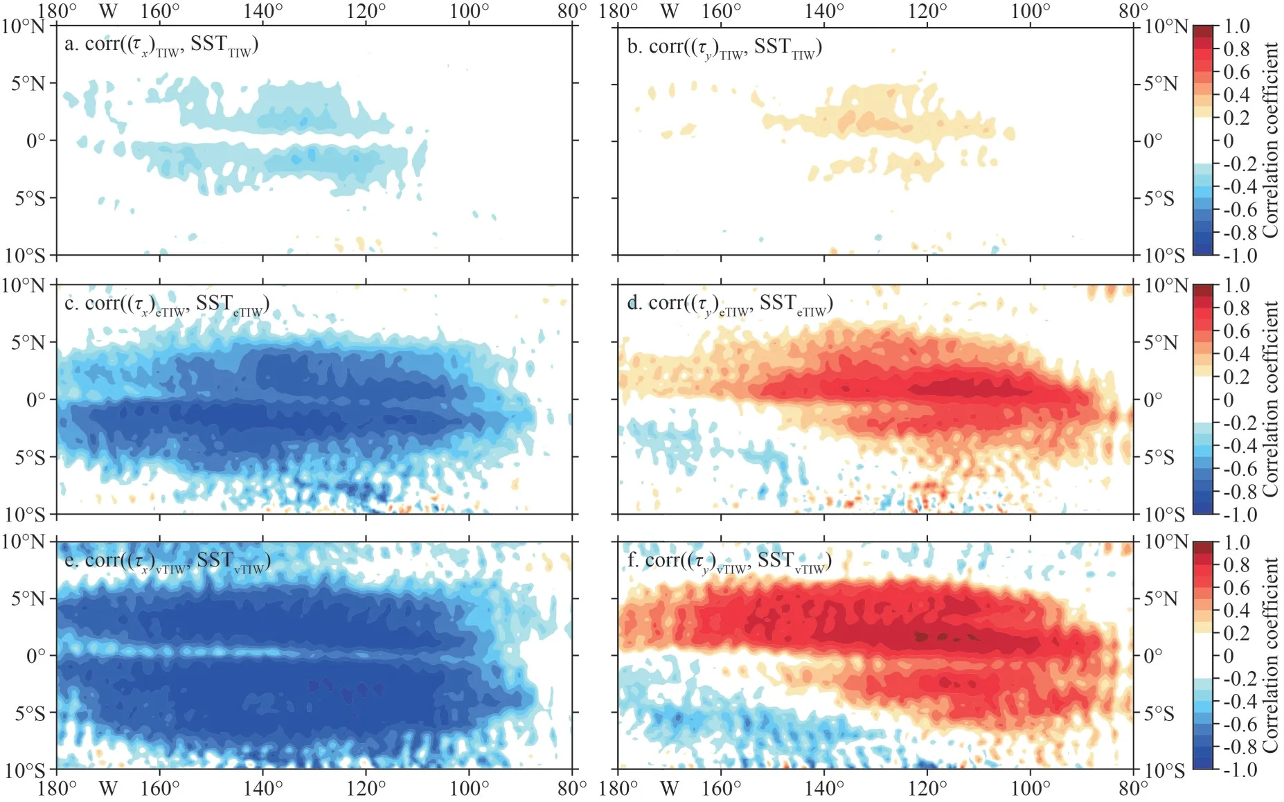
Fig.4 Correlation coefficients between the SSTTIW and τTIW from 2008 to 2019 in the Eastern Pacific (180°-80°W, 10°N-10°S)

We get the regression coefficients and show them in Fig.5.In the regions where the TIWs are active,the absolute values of regression coefficientsaxandayare about 0.01-0.02 N/(m2·°C), which have the same range as the coefficientsbxandbyon vTIW.These results are similar to that derived by Maloney and Chelton (2006), O’Neil et al.(2010), and Wei et al.(2018).However, the air-sea coupling strength induced by vTIW is stronger than that by eTIW in the most regions, with an exception that the coupling strength caused by eTIW is stronger in the equatorial region, which may be determined by the distributions of the two modes of TIWs: the eTIW is centered at the equator, while the vTIW is centered at 4°N and the range is wider.Furthermore, the region of high regression coefficientsaxandbxare much larger thanayandby, which shows roughly the same pattern as the correlation coefficients in Fig.4.Therefore, we confirm that the coupling relationships obtained by Pezzi et al.(2004) and Wei et al.(2018) remain when eTIWs and vTIWs are considered separately, but reveal that the coupling coefficients for individual TIW modes are stronger than combining them.

Since previous studies have confirmed that TIWs have seasonal characteristics, and they are more active in autumn and winter, we verified that the coupling relationships betweenτTIWand SSTTIWalso has monthly variations during these active months(Fig.6).In general,bxandbyare significantly stronger thanaxanday, indicating that the air-sea coupling relationship induced by vTIW is stronger than that of eTIW.However,ayare significantly smaller thanbywith almost constant difference, the same significance relationship does not exist betweenaxandbx.The monthly variations ofayandbyare weak,and they fluctuate slightly around the mean value of 0.01 N/(m2·°C).In contrast,axandbxfluctuate greatly, with the smallest coupling strength in October and the largest in January, which has not been pointed out in previous studies.

3.2.2 Coupling model between the gradient of SSTTIWand divergence (curl) ofτTIW

For the convergence-divergence center juxtaposed with the SST gradient maxima observed in Fig.2,Chelton et al.(2000) pointed out that the effects of SSTTIWon the overlyingτTIWdepend on both the SSTTIWgradient and the wind direction relative to the SSTTIWgradient.There is therefore no general linear relation between the gradient ofτTIWand the SSTTIWgradient.TheτTIWresponses to the geographical variations of the underlying SSTTIWfield therefore can be better characterized in terms of (divτ)TIWand(curlτ)TIW(Fig.7).

Fig.6 Seasonal variation of the regression coefficient (unit:N/(m2·°C)) in active months of eTIW and vTIW

Fig.7 The composite SSTeTIW and the divergence and curl of τeTIW in active months from 2008 to 2019

The (divτ)eTIWshown in Fig.7 are mainly distributed in the boundary between the cold and the warm anomalies, which reflects the feedback ofτeTIWto SSTeTIW: a monopole of SSTeTIWcorrespond to a dipole (divτ)eTIW, suggesting DMT mechanism is dominant (Chelton et al., 2004).The largest (divτ)eTIWis located directly over the strongest SSTeTIWgradients.It is visually apparent that the (divτ)eTIWis locally larger where the wind is aligned perpendicular to isotherms of SSTeTIW(i.e., parallel to the SSTeTIWgradient).

Chelton et al.(2000) hypothesized that the SST modification of the wind stresses can be independently evaluated from the relationship between the crosswind SST gradient and curl.The (curlτ)eTIWtakes larger values where the wind blows parallel to the isotherm(that is, perpendicular to the SSTeTIWgradient vector;Fig.7c).As shown in Fig.7c, there are indeed large(curlτ)eTIWcenters at the southern boundaries of both the cold and warm anomalies: the southern boundary of the cold SSTeTIWcorresponds positive (curlτ)eTIW,and the warm SSTeTIWboundary corresponds negative(curlτ)eTIW.Over the warm water, because of the shear between the higher speeds to the right and lower speeds to the left of the air parcel, a negative curl is generated when the wind blow along the SSTTIWisotherms of the southern edge.This makes a significant linear relationship between (curlτ)TIWand crosswind SSTTIW.

Therefore, the correlations between (divτ)TIWands·?SSTTIW(SSTTIWgradient following the direction of the original wind), and between (curlτ)TIWandn·?SSTTIW(SSTTIWgradient perpendicular to the wind)were obtained, respectively.sdenotes the unit vector in the direction of wind stress andnthe unit vector obtained after 90° counterclockwise rotation ofs.The absolute values of the correlation coefficients between ?SSTeTIWand (divτ)eTIW((curlτ)eTIW) are all ＞0.4, but the correlation in eTIW is slightly smaller than that in vTIW (Fig.8a-b).The correlation coefficients have the largest values on the east side of the equator and gradually decrease towards north and south, which is similar in eTIW and vTIW, and the distributions on both sides of the equator are basically symmetrical.However, the high correlation coefficients in the vTIW scale have wider latitude bands.

Since the above correlation coefficients have passed the significance test in the regions where the TIWs are active, in these regions, regression models(Eq.4) can be developed between (divτ)TIWands·?SSTTIW, and between (curlτ)TIWandn·?SSTTIW:

The obtained regression coefficients for every points in this region are shown in Fig.9.Being about the same as vTIW,a1ranges 0.02-0.03 N/(m2·°C)south of the equator and 0.01-0.02 N/(m2·°C) north of the equator, whilea2has smaller values around 0.01 N/(m2·°C) in both sides of the equator.Comparing eTIW with vTIW, the regression coefficientsa1is slightly larger thanb1near the equator, but smaller in other regions.a2andb2have similar values(Fig.10c-d).The distributions of the regression coefficients with approximately symmetrical structures are basically the same as the correlation coefficients in observations, but smaller spatial scale in eTIW than vTIW.In this study, the previous research results are decomposed into eTIW and vTIW groups, and the regression coefficients obtained respectively have obvious differences, so the models in this study are more targeted and could better describe the relevant sea-air interactions.

It is worth noting that the response of (divτ)TIWtos·?SSTTIWis larger than that of (curlτ)TIWton·?SSTTIW.This phenomenon has been described previously, O’Neill et al.(2010) explained it statically, and suggested that it is resulted from gradients of the frontally induced surface wind direction that diminished the wind stress curl but enhanced the wind stress divergence, thus the response of divergence is more intense.In addition,Schneider and Qiu (2015) explained dynamically that when the wind is parallel to the SST front, a larger wind stress curl is expected to be reduced by the geostrophic spin down, resulting in a small coupling coefficient.These expressions, as well as Fig.9, illustrate this phenomenon and its plausibility of existence.

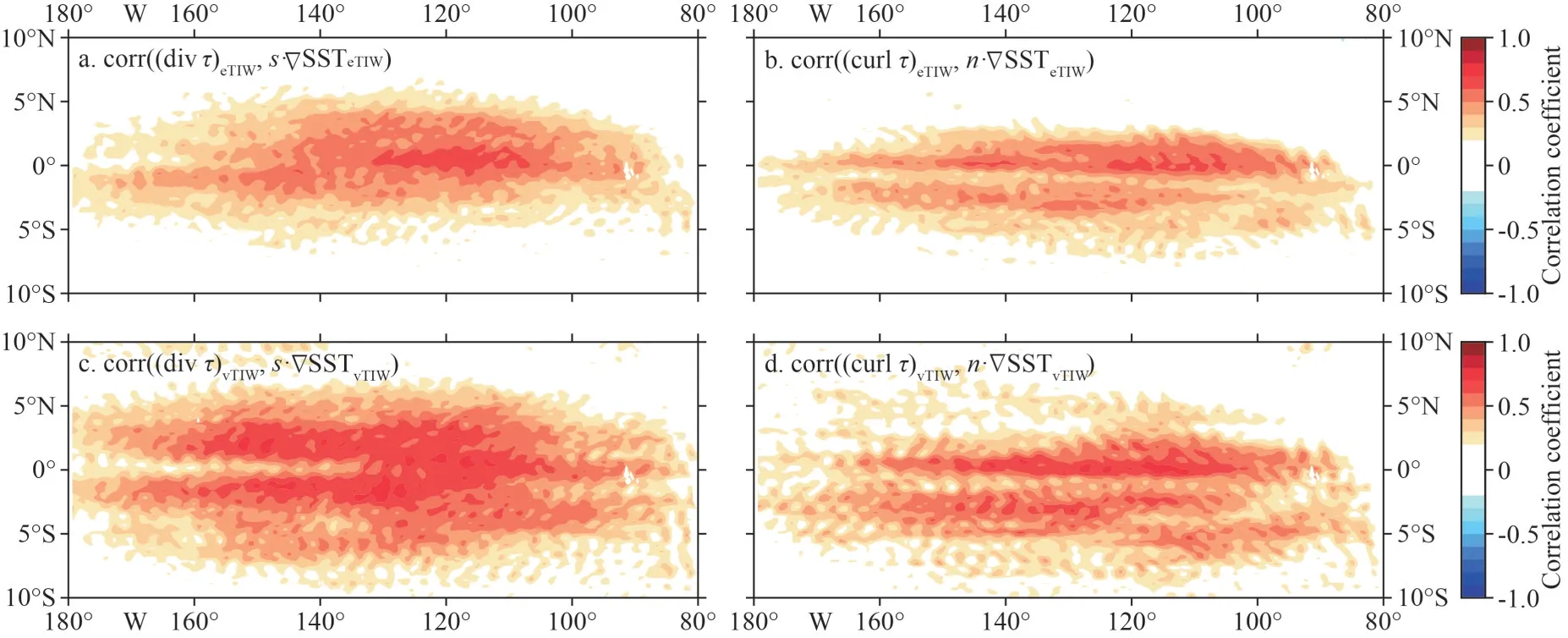
Fig.8 Correlation coefficients between the SSTTIW and the (div τ)TIW ((curl τ)TIW) from 2008 to 2019 in the Eastern Pacific(180°-80°W, 10°N-10°S)

Fig.9 Regression coefficients (unit: N/(m2·°C)) of SSTTIW gradient and τTIW field from 2008 to 2019 in 180°-80°W, 10°S-10°N

Fig.10 Differences between eTIW- and vTIW-induced regression coefficients (unit: N/(m2·°C)) from 2008 to 2019 in 180°-80°W, 10°S-10°N

In summary, we investigate the coupling relationship betweenτTIWand SSTTIWinduced by bimodal TIWs, using SST data and wind stress data from 2008 to 2019.Compared with previous studies,we separate the TIWs into eTIW and vTIW.We discover that such air-sea interactions in previous studies still exists in both eTIWs and vTIWs, but with noticeable differences.We also find that there are more significant correlations between their individual inducedτTIWand SSTTIWthan the combining TIWs.Besides, vTIW-induced correlations and coupling strengths are stronger than eTIW in most areas (Fig.10a-b).As eTIW and vTIW have different properties, their induced air-sea interactions are also different; e.g., eTIW is centered at the equator, so the coupling strength is stronger than vTIW at the equator.Due to the larger areas where vTIWs occur than eTIWs,the resulted strong air-sea interaction also has larger spatial scales, especially in the latitude range.

The significant linear relationship between SSTTIWandτTIWalso indicates that the larger the SSTTIW, the larger theτTIW.The SSTTIWinduced by eTIW and vTIW is about 0.2-0.3 °C after long-term composite; and the correspondingτTIWis around 0.002-0.006 N/m2,which has been examined to have a substantial effect on modulating long-term mean state in the equatorial Pacific (Pezzi et al., 2004; Zhang and Busalacchi, 2008; Wei et al., 2019).In addition, we confirm thatτTIWalso plays a significant role in the short-term average: we chose September 1-7 in 2008(same as Fig.1) for an example, the proportion of averaged -- ---τTIW/τˉ are roughly 5%-15% in the areas where TIWs are active (not show here).Therefore,theτTIWhave strong feedback effects on the ocean.

4 BIMODAL TIW-INDUCED AIR-SEA COUPLING IN OCEAN GENERAL CIRCULATION MODELS

According to previous studies, TIW-induced airsea interaction plays an important role in both ocean and atmosphere.Wei et al.(2018) revealed that TIWinduced wind stress perturbations have a substantial effect on the equatorial Pacific heat budget.In Section 3, we reveal thatτTIWaccounts for a nonnegligible proportion of the wind stress, which surely will influence the bimodal TIWs and ocean mean state.Thus, it is necessary to investigate how the representative ocean circulation models and coupled climate models (Section 5) can represent the eTIW- and vTIW-induced air-sea interactions.

4.1 Air-sea coupling induced by bimodal TIWs in the HYCOM model

The SSTTIWandτTIWin HYCOM are shown in Fig.11a-b.In comparison with the compositeτTIWand SSTTIWin observations (Fig.2), this model is able to reproduce the patterns of SSTTIWnorth of the equator but with slightly lower values (less than 0.1 °C).Yet the spatial pattern south of the equator of SSTTIWis not well simulated.In addition, the HYCOM model cannot clearly display the spatial correspondences between SSTTIWandτTIW.

To investigate how the HYCOM can represent these interactions.The first approach is to evaluate the correlation between SSTTIWand the two components ofτTIW(Fig.11c-f).The second is to evaluate the correlations between the derivative fields ofτTIWand the gradient of SSTTIW(Fig.11g-j).In contrast to the correlation coefficients derived from the observations shown in Figs.4 & 8, this model cannot well characterize the correlations between SSTTIWandτTIW.Moreover, the distributions of the correlation coefficients are very scattered, and no specific distribution patterns like the observations are found.

In fact, HYCOM seems not to well simulate either eTIWs or vTIWs.Regression analysis was no longer performed due to the extremely low correlation coefficients.Although HYCOM is a highly sophisticated and advanced ocean model that incorporates observations, it still seems to suffer from shortcomings that can be attributed to errors in the atmospheric forcing, such as the implausibility of the wind stress bulking formula it uses.

4.2 Air-sea coupling induced by bimodal TIWs in the ECCO2 model

Comparing the SSTTIWandτTIWof the ECCO2 model(Fig.12a-b) with observations (Fig.2), it demonstrates that ECCO2 can well present the patterns of SSTTIWon both sides of the equator that are active between 5°S-5°N, although values are slightly larger than the satellite observations.In addition, a clear spatial correspondences between SSTTIWandτTIWcan be observed with accelerated wind stress in the SST anomaly region;τTIWpoints to the northwest over warm water and southeast over cold water; which are similar to the conclusions in Fig.2.

The correlations between SSTTIWandτTIWare significant, so we will not show them but the regression coefficients only (Fig.12c-j).Spatially,the distributions of the regression coefficients for two models are basically consistent with the observations within the meridional band 8°S-8°N.Nevertheless, the distributions of regression coefficients for (curlτ)TIWandn·?SSTTIWare wider than the observations, especially for the eTIW.In satellite observations, the distributions of the regression coefficients for (divτ)TIWands·?SSTTIWare more restricted than that for (curlτ)TIWandn·?SSTTIW.However, in ECCO2, the latter has a larger latitude span.In addition, the air-sea interaction caused by vTIW is stronger than that caused by eTIW, which is mainly reflected in the spatial scales.

These regression coefficients in the eastern tropical Pacific are about 0.001-0.002 N/(m2·°C) in the first methods (Fig.12c-f), and about 0.002-0.004 N/(m2·°C) in the second method (Fig.12g-j).The values are lower than observations coherently.Notably, the response of (curlτ)TIWton·?SSTTIWis similar to the response of (divτ)TIWtos·?SSTTIWin ECCO2, which is the most obvious difference from observations.

In general, ECCO2 shows a good performance in simulating both the eTIWs and vTIWs; it also fully depicts the air-sea interactions induced by them.This may be due to the superiority that the forced wind field used in ECCO2 has been optimized(Menemenlis et al., 2008), so it is more consistent with the observations and has better performance.

5 THE BIMODAL TIW-INDUCED AIRSEA COUPLING IN FULLY COUPLED CLIMATE MODELS

In this section, we further investigate how well the coupling relationships remained in several widely recognized fully coupled climate models,with a focusing on the effect of model resolution on the final performance.

5.1 Air-sea coupling induced by bimodal TIWs in the CESM2-FV2 model

Fig.12 The composite map and regression coefficients (unit: N/(m2·°C)) in ECCO2 model from January 1, 2009 to December 31, 2017

The composite of SSTTIWandτTIWof CESM2-FV2 during active months are shown in Fig.13a-b.In comparison with theτTIWand SSTTIWin observations (Fig.2), the bimodal TIW-induced SSTTIWare active between 5°S and 5°N in equatorial asymmetry, which is similar to the observations;however, values of SSTeTIWin this model (around 0.1 °C) are smaller than those of observations(around 0.2 °C).The spatial correspondences between SSTTIWandτTIWare consistent with the observations,but the values ofτTIWare about 10 times smaller.Another difference is that the direction of wind stress is deflected from observations south of the equator.

The regression coefficients are shown in Fig.13c-j.Spatially, the distributions of the effective regression coefficients are similar to the observations, mainly concentrated in 8°S-8°N, 180°-80°W.Differently,in the south of equator, the regression coefficients of(τy)TIWand SSTTIWare mainly concentrated in the west of 140°W in observation, while they in the CESM2-FV2 model mainly exist east of 120°W with the opposite sign.Furthermore, this model fails to reproduce the observed symmetrical distribution patterns of the regression coefficients of the second method.

Fig.13 Same as Fig.12, but for CESM2-FV2 mode from January 1, 2000 to January 1, 2015

The regression coefficients in most areas are about 10 times smaller than the observations’; only in a small part of the southern hemisphere (Fig.13c,d, g, & i), this model shows comparable regression coefficients to the observations.Furthermore, the first coupling relationships induced by eTIW and vTIW are comparable, while the second coupling relationship on eTIW is stronger than on vTIW.

5.2 Air-sea coupling induced by bimodal TIWs in the CESM2-WACCM model

From the compositeτTIWand SSTTIWof this model shown in Fig.14a-b, we can judge that the simulation of CESM2-WACCM is better than that of CESM2-FV2.The spatial patterns are consistent with the satellite observations.The values ofτTIWand SSTTIWare smaller, but is closer to the satellite observations than CESM2-FV2.Other features in Fig.14a-b are similar to CESM2-FV2.

Spatially, the distributions of the regression coefficients (Fig.14c-j) are similar to the observations(Figs.5 & 9), mainly concentrated between 8°S-8°N,180°-80°W.Moreover, the regression coefficients of(τy)TIWand SSTTIWare asymmetric about the equator,the regression coefficients of (τx)TIWand SSTTIWand of the second method are approximately symmetrical structures, which are consist with observations.The spatial scales in eTIW are smaller than that in vTIW.

Fig.14 Same as in Fig.12, but for CESM2-WACCM mode from January 1, 2000 to January 1, 2015

The regression coefficients of the first method are slightly smaller than the observations (Fig.5) in most regions, but larger coefficients appear on the northern edge.The coefficients of the second method(Fig.14g-j) are well simulated south of the equator,but are still about 0.01 N/(m2·°C) smaller than observations’ (Fig.9).As with CESM2-FV2, the modelling of the second coupling relationships north of the equator is weaker.Overall, this model performs well in the simulation of the relationship betweenτTIWand SSTTIW.

Comparing with CESM2-FV2, the regression coefficients of two methods in CESM2-WACCM are slightly stronger (Fig.14c-j), which is probably due to its higher spatial resolution or the superiority of the WACCM6 atmospheric mode.This issue will continue to be discussed in Section 5.3.

5.3 Air-sea coupling induced by bimodal TIWs in the CESM2-WACCM-FV2 model

CESM2-WACCM-FV2 can well depict the spatial patterns of composite SSTTIWandτTIWnorth of the equator (Fig.15a-b).However, south of the equator,the anomaly areas of SSTTIWare larger than the areas in observations (Fig.2).The spatial correlations betweenτTIWand SSTTIWare obvious, but a little direction deflection ofτTIWin the south of equator.The values of SSTTIWandτeTIWare about twice smaller than observations whileτvTIWare almost the same as the observations’ in value.

The regression coefficients of two methods are shown in Fig.15c-j.The spatial distributions of regression coefficients are mainly concentrated between 8°S-8°N and 180°-80°W, which is similar to the observations’.The largest deviation is consistent with the CESM2-FV2 and appears in the regression coefficients of (τy)TIWand SSTTIW.Furthermore, this model fails to display the observed symmetrical distributions of others regression coefficients, spatial scales south of the equator are smaller.

The values of regression coefficients are similar to CESM2-FV2, but about 10 times smaller than the observations’.However, the absolute values are almost symmetrical about the equator.The two coupling relationships are stronger induced by vTIW than by eTIW.

Fig.15 Same as in Fig.12, but for CESM2-WACCM-FV2 mode from January 1, 2001 to December 31, 2014

Comparing the above three models, CESM2-WACCM-FV2 has the same atmospheric model as CESM2-WACCM, but lower spatial resolution.Besides, the spatial resolutions of CESM2-WACCMFV2 are the same as CESM2-FV2, but different from those of atmospheric models.The regression coefficients of CESM2-WACCM-FV2 are basically the same as the CESM2-FV2, but lower than CESM2-WACCCM.Therefore, it can be inferred that regression coefficients may be related to resolution.

In addition, the biggest difference from observations exists in the regression coefficients between (τy)TIWand SSTTIW: the coefficients are negative south of the equator, contrary to satellite observations, especially in CESM-FV2 and CESM2-WACCM-FV2.It is noted that the common difference between these two models and CESM2-WACCM is the coarser horizontal resolution of 1.9°×2.5°.Consequently, we can again conclude that such deviations of simulations are more likely caused by the coarse resolutions.

Through the comparisons of the above three modes, it is inferred that the performance of the simulation in the coupling between SSTTIWandτTIWcan be closely related to the spatial resolution of the atmospheric models.The higher resolution corresponds to more realistic simulation.Thus, the climate model air-sea coupling deficiencies may therefore be partially ameliorated by increasing the grid resolution of the atmosphere models.

5.4 Air-sea coupling induced by bimodal TIWs in the MPI-ESM1-2-HR model

The spatial patterns of SSTTIWin this model(Fig.16a & b) are significantly different from the patterns in satellite observations (Fig.2), with a “＜”shape north of the equator, which is quite different from the pattern of bimodal TIWs in previous studies(Xie, 2004; Wei et al., 2018).The values of SSTTIWandτTIWare much smaller than observations.However, the spatial correspondences between SSTvTIWandτvTIWare well depicted: the areas with large SSTvTIWhave largeτvTIW; theτvTIWover the warm water is northwestward,and over the cold water is southeastward.

Spatially, in general, the spatial scales of the regression coefficients in this model are obviously smaller than in observations (Figs.5 & 9).The performance in simulating the air-sea coupling relationships in eTIW is worse than that in vTIW.The regression coefficients of the first method are mainly distributed north of the equator on the eTIW scale, but are distributed both north and south on the vTIW scale.The regression coefficients of the second method only exist in an extremely small area north of the equator on eTIW scale, while have larger spatial scales both north and south with larger value in vTIW.Numerically, the values are less than 0.000 5 N/(m2·°C), only the regression coefficients of (divτ)TIWands·?SSTTIWare larger, but still less than 0.01 N/(m2·°C).

In short, MPI-ESM1-2-HR has a poor performance in simulating both eTIW and vTIW, it also fails to produce bimodal TIW-induced air-sea coupling interactions.

5.5 Air-sea coupling induced by bimodal TIWs in MPI-ESM-1-2-HAM

Finally, the performance of MPI-ESM-1-2-HAM model is examined.The spatial patterns of SSTTIWare simulated better than MPI-ESM1-2-HR, but the values ofτTIWare too small (Fig.17a-b).There is no apparent spatial or temporal correlations between SSTTIWand (τx)TIW((τy)TIW), which is also visualized in Fig.17c-f.Moreover, there is no obvious spatial correlation between ?SSTTIWand (divτ)TIWor (curlτ)TIW(as shown in Fig.17g-j).

The signs of the correlation coefficients are consistent with the observations (Figs.4 & 8): (τx)TIWand SSTTIWare negatively correlated, and the rest are positively correlated.However, all the correlation coefficients are not large enough for regression analysis.Besides, the simulation on the eTIW scale is a little better than that on the vTIW, with larger coefficients and larger spatial scales.The significant coefficients in eTIW are mainly distributed near the equator with low correlations (|R|＜0.4).

In conclusion, the MPI-ESM-1-2-HAM also shows low capability in simulating the bimodal TIWs and the corresponding air-sea interactions.

The results meet the expectation that the coupling strengths in coupled climate models are usually weaker than those in the satellite observations,mainly due to their low resolutions, which cannot catch the coupling well (Maloney and Chelton,2006; Bryan et al., 2010).

6 DISCUSSION AND CONCLUSION

Fig.16 Same as in Fig.12, but for MPI-ESM1-2-HR mode from January 1, 2000 to December 31, 2014

Using the latest high-resolution satellite observations,we have constructed the relationships between the two modes of TIWs and their induced fluxes at the air-sea interface, i.e., the relationships between SSTTIWandτTIW.Based on previous studies, we distinguished two modes of TIWs, which is the main part of innovation of this study.To quantify the coupling relationships, we used two methods mainly.The first is to establish the relationship between SSTTIWand the components ofτTIW.The second is to establish the relationship between (divτ)TIW((curlτ)TIW)ands·?SSTTIW(n·?SSTTIW).Thus, we established two empirical coupling models.Previous studies have shown a significant relationship between wind stress and SST perturbations caused by undifferentiated TIWs, but did not explore whether the relationship exists in bimodal TIWs or whether differences exist between eTIW- and vTIW-induced.In this study, we confirmed that when dividing TIWs into eTIW and vTIW, the coupling relationships still exist between their individual induced SST and wind stress, the coupling coefficients are similar to the previous studies.However, the correlations are higher than combining them, so the linear relationships between the variables are stronger and the regression models fit better than in previous studies.

In addition, we investigated the correlations between SSTTIWandτTIWin several widely accepted ocean general circulation models and fully oceanicatmospheric coupled climate models.By comparing the results obtained from satellite observation, we confirmed that the coupling relationships produced by the models are weak and insufficient, which may bring uncertainties when using these model data for some studies.In addition, we also found that the ability to simulate coupling relationships is tied to spatial resolution.Clearly, the bias of the simulation is smaller in the high-resolution model.The air-sea interactions induced by both eTIWs and vTIWs in numerical model with higher resolution atmospheric model matched better with satellite observations.

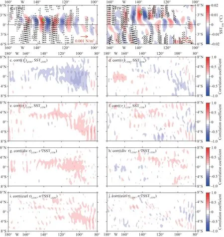
Fig.17 Same as in Fig.11, but for MPI-ESM-1-2-HAM mode from January 1, 2000 to December 31, 2014

The empirical coupling models of two methods established in this study effectively represent the airsea interactions on eTIW scale and vTIW scale.In the future, it can also be used in either oceanic or couple models (Pezzi et al., 2004; Zhang and Busalacchi, 2008, 2009).Besides, the coupling model of (divτ)TIW((curlτ)TIW) and downwind (crosswind)?SSTTIWis convenient for separating the wind stress divergence-only and curl-only components.It has been revealed that both the divergence-only and curl-only wind stress can bring changes on the ocean (Wei at al., 2019).Curl always regarded as a critical factor that influences the ocean (Chelton et al., 2001; Milliff et al., 2004; Hogg et al., 2009).However, the function of divergence has been overlooked.This model can separate divergence to facilitate the study of its individual effects on the ocean.

The series models released by both NCAR and MPI reveal that the TIW-induced interactions are highly dependent on the horizontal resolution of the model; higher resolution corresponded to more accurate coupling, suggesting the importance of adequate resolution for simulating realistic air-sea interactions on bimodal TIW-scales.It is inferred that increasing the resolution of the model is a feasible way to improve the performance of simulation.Moreover, we found some of the models failed to reproduce these coupling relationships; the behind reasons were not investigated,but deficiencies in the parameterization of air-sea interface physics likely contribute to some of the differences between these models and observations(Spall, 2007; Song et al., 2009; Chelton and Xie, 2010).

A complete picture of the air-sea interactions should include the SST-wind stress interactions induced by eTIW and vTIW.The ability of numerical models to properly represent air-sea coupling induced by both eTIW and vTIW have significant implications for realistic simulation of the atmosphereocean climate system.That is to say, the coupling models in this paper can not only be used to evaluate the performance of the models on the bimodal TIWs scales, but also can be used to improve the whole air-sea coupling relationships of the models.

However, we only investigated the relationship between SST and wind stress perturbations induced by bimodal TIWs, some intermediate process in the interaction between wind stress and SST remain unrevealed (Jin et al., 2009).We should analyze these intermediate processes in future studies to support the conclusions of this study.Moreover, the true coupling relationship involves more atmospheric processes, which also need to be studied to establish a more comprehensive coupling relationship.

7 DATA AVAILABILITY STATEMENT

All data analyzed in this study are publicly available.The NOAA OISST V2 high resolution dataset data provided by the NOAA PSL, Boulder, Colorado, USA,from their website at https://psl.noaa.gov.The ASCAT data are produced by Remote Sensing Systems and sponsored by the NASA Ocean Vector Winds Science Team, data are available at www.remss.com.The HYCOM data was funded by the U.S.Navy and the Modeling and Simulation Coordination Office, and was made available by the DoD High Performance Computing Modernization Program.The output is publicly available at http://hycom.org/.The ECCO2 data are available at http://apdrc.soest.hawaii.edu/data/.The data from the CMIP6 were downloaded from https://esgf-node.llnl.gov/projects/cmip6/.

8 ACKNOWLEDGMENT

We thank the working groups responsible for the above datasets.