Numerical analysis for the free-boundary current reversal equilibrium in the AC plasma current operation in a tokamak

Yemin HU (胡業民),Liuqing WANG (王柳青),Shuhang BAI (白書航),Zhi YU (于治) and Tianyang XIA (夏天陽)

1 Institute of Plasma Physics,Chinese Academy of Sciences,Hefei 230031,People’s Republic of China

2 University of Science and Technology of China,Hefei 230026,People’s Republic of China

3 Institutes of Physical Science and Information Technology,Anhui University,Hefei 230601,People’s Republic of China

Abstract In recent decades,tokamak discharges with zero total toroidal current have been reported in tokamak experiments,and this is one of the key problems in alternating current (AC) operations.An efficient free-boundary equilibrium code is developed to investigate such advanced tokamak discharges with current reversal equilibrium configuration.The calculation results show that the reversal current equilibrium can maintain finite pressure and also has considerable effects on the position of the X-point and the magnetic separatrix shape,and hence also on the position of the strike point on the divertor plates,which is extremely useful for magnetic design,MHD stability analysis,and experimental data analysis etc.for the AC plasma current operation on tokamaks.

Keywords: current reversal equilibrium,AC operation,free-boundary equilibrium,tokamak

1.Introduction

Alternating current (AC) operation of a tokamak reactor is an attractive way to generate a continuous output of electric energy without the need for a complicated non-inductive current driving system.In recent decades,AC operation experiments have been performed in a number of tokamak devices [1-11].This approach has been demonstrated to be feasible and free from secular degradation in performance.AC tokamak operation is always associated with a magnetic equilibrium in which the current density reverses.It is well known that the first step in tokamak modeling and analysis is the reconstruction of MHD equilibrium and stability calculations.Some active theoretical research activities on the current reversal equilibrium configurations (CRECs) have been done analytically [12-14] and numerically [15-17].However,previous research mainly focused on the existence of the CRECs [12,13,15] and the fixed-boundary CRECs[12,14,15,17],which are important for the understanding of the physics of CRECs but invalid for practical application to experiments on the CRECs reconstruction calculations to determine the magnetic separatrix and X-point locations.In practical experimental equilibria,the position of the plasma boundary is determined by the interaction between the currents in plasmas and in the plasma equilibrium control coils.For the current reversal equilibrium configuration,the plasma magnetic surface is not nested,and the magnetic surface function is not suitable for normalization by the poloidal magnetic flux at the magnetic axis and plasma boundary.It is highly difficult to adjust the plasma current profile using the iterative method adopted by Johnsonet al[18] when the macroscopic plasma parameters are known.Therefore,we must use the finite element method of unstructured mesh and transform the free boundary problem into a series of fixed boundary problems to deal with,that is,the Hagenow and Lackner method [19-21].

In this paper,we propose an improved Hagenow and Lackner method through which the current reversal equilibrium configuration and the external control coil current can be obtained from the prescribed plasma parameters in the tokamak configuration with plasma surface bounded by a given desired plasma shape or the X-point outside of the torus.In section 2 we describe the plasma equilibrium model and the method of solution.In section 3,the benchmark and some results related to the actual plasma shape are presented for equilibria with current reversal.The summary and conclusions are described in section 4.

2.Numerical methods of solving the Grad-Shafranov equation with free boundary conditions

The ideal MHD equilibrium in an unbounded domain can be described by a second-order partial differential equation,i.e.the so-called Grad-Shafranov equation.In axisymmetric geometry,it can be written in cylindrical coordinates (x,?,z)as follows [18,21]:

with

When the plasma is surrounded by a vacuum region,j?is nonzero only in the interior of the plasma.We assume that the plasma is in a domain of the cross-section denoted by Ωp,with boundary Γp,and the outside of the plasma is a vacuum region denoted by Ωvwith a rectangular computational boundary Γv.It is worth noting that for the free boundary current reversal equilibrium,the poloidal magnetic flux within the plasma region is non-nested and not monotonic,so the boundary of the plasma and vacuum cannot be determined by comparing the value of the poloidal magnetic flux with a given ψΓpas was done in reference [18],which is widely used by EFIT and other codes etc.In addition,when we want to effectively optimize the plasma current profile to improve the convergence efficiency of the solver,the poloidal magnetic flux at this time cannot be normalized simply as done in reference [18],that is to say,their method does not work efficiently in this case.However,we extend the method of Hagenow and Lackner,and find that it may be an efficient method for the solution of the CREC of equation (1) in an unbounded domain.The solution process can be grouped in the following steps:

Step 1.Determinej?(x,ψ) by solving equation (1) in the plasma region imposed the Dirichlet conditions along a given closed curve Γp,with ψ on Γpgiven as a constant ψΓp.

Equation (1) is a nonlinear equation,and both β andfare general functions of ψ.Without the loss of generality,considering ψΓp=0 ,we take the profiles of β andfas the following polynomial of ψ:

with the same boundary condition as in equation (1) with a toroidal current densityj?=λψ/x,and comparing with equation (2) we can obtain.An equilibrium solution with the nested flux surfaces ψ=const corresponds to the lowest eigenvalue and an eigenfunction without nulls inside the plasma domain.A lot of other eigenfunctions provide a series of equilibria with a different topology of the magnetic surfaces.

Step 2.Construct the Green’s function of the Grad-Shafranov operator to solve equation (1) in an unbounded domain.

The known Green’s function in a cylindrical geometry is given by the following [22]:

whereGsatisfies

whereK(k) andE(k) are complete elliptic integrals of the first and second kind,and (x′,z′) is the observation point.Using Green's theorem gives

We integrate the above equation over all space and use Gauss’s theorem to convert the divergences to surface integrals which vanish at infinity,then the expression to obtain ψoutside or on the computational boundary is

From the above equation (13),it is clearly found that ψ is composed of the magnetic fluxes induced by the plasma current (the first term on the right hand side (RHS)) and the external coil currents (the second term on the RHS).

Step 3.Compute the contribution from the plasma currents using the von Hagenow method.

Consider a function ψg(x,z) which satisfies the same differential equation as equation (1) that ψ does in the interior of the rectangular computational boundary Γv,but which vanishes on the boundary,i.e.:

The resulting flux-function distribution ψgcan be interpreted as the sum of the field induced by the plasma currents plus the field of the fictitious mirror currents in an unbound domain.In order to solve equation (14) efficiently,we can use interpolation to transformj(x,ψ) intoj(x,z),and equation (14) becomes a linear partial differential equation with very good convergence performance.In the same way as in step 2,we use the following form of Green's theorem:

Integrating the above equation over the computational domain Ωc=Ωv+Ωp,using ψg|Γv=0,and evaluating the differential surface element related to the differential line element by dS=2πxdl,then we can obtain the identity as follows:

The second term on the RHS of the above equation represents the fictitious mirror currents in an unbound domain.Substituting equation (17) into equation (13) yields [20]

which is the solution of equation (1) at a point interior to the computational boundary.

Step 4.Determine the external coil currents to produce a given plasma shape.

To determine the necessary external currents,we solve the overdetermined problem of finding the least square error[21,23-25] in the poloidal flux at theNkplasma boundary pointsproduced byNccoils at set locationswithNk＞Nc.Assuming that the plasma boundary points lie interior to the computational boundary,we use equation (18)to express the function to be minimized as

where

Here γ1and γ2are the regularization parameters which are introduced to stabilize the procedure against large unreal oscillations of the currentIiand the dramatic current change of adjacent coils; and ψbis the desired value of flux at the given boundary points.We minimize ? by ??/?Ii=0,and obtain

The above algebraic equation can be rewritten in a concise form as follows:

Finally,we summarize the equilibrium algorithm in figure 1.Initially,we guess a profile for the plasma current.We use this to give a first guess for the desiredIp0,βv0within the desired plasma boundary shape using equations (6)and (4).With these constraints held fixed,we solve equation(1) with fixed plasma boundary.When this converges,we use the current distribution so computed to obtain the poloidal magnetic flux ψ by solving equation (14) with the rectangular computational boundary and its corresponding adjoint Green's function.Secondly,we use the magnetic flux obtained above and the desired boundary flux value,by adjusting parameters γ1and γ2,hold the boundary flux fixed until convergence,and finally determine the coil current in the vacuum outside the plasma.

3.Benchmark and free-boundary CRECs simulation

3.1.Benchmark

According to the above detailed solution process,we developed an Advanced Tokamak Equilibrium Code (ATEC),which is written in MATLAB language.The Grad-Shafranov (G-S) operator solver is from the PDE solver in the MATLAB toolkit.The computational domain is discretized by a triangular mesh finite element method.We directly call the function “initmesh” in the MATLAB mathematical function library to generate triangular mesh,and call the nonlinear PDE solver function “pdenonlin” to solve the nonlinear G-S equation.This code was benchmarked against the wellknown equilibrium code EFIT [26] and TEQ [27] for the normal nested plasma equilibrium configuration.An example of the comparison between the equilibrium results from EFIT,TEQ and ATEC is shown in figure 2,where the plasma parameters,profiles and related equilibrium information all come from the EAST equilibrium data file g070754.003740 calculated by EFIT and the CFETR equilibrium data file g220905.7500_teq calculated by Tequation.The position,size,and turns of the poloidal coils come from table 1 in references [28] and [29].The red lines in figure 2 are the results from ATEC using coil currents given by EFIT(a),ATEC (b) itself for EAST,and TEQ (c),ATEC (d) itself for CFETR.The blue dashed lines in figure 2 are the results from EFIT for EAST ((a) and (b)) and TEQ for CFETR ((c)and (d)).It can be found that the results of ATEC and the other two codes are in good agreement.Tables 1 and 2 show the comparison of the coil currents,the total coil currents,and the errors of the last closed flux surface (LCFS),X-point and magnetic axis calculated by the codes ATEC,EFIT,and TEQ for EAST and CFETR,respectively.

3.2.Free-boundary CRECs simulation

Figure 2.Comparison of the magnetic surface calculation results of ATEC,EFIT,and TEQ.Blue: EFIT and TEQ,red: ATEC; EAST:(a) using coil current by EFIT,(b) using coil current by ATEC; CFETR: (c) using coil current by TEQ,(d) using coil current by ATEC.

In the following section,the second type of free boundary case is considered,and the plasma parameters for simulation are from the EAST data of shot # g070754.003740.The desired LCFS is also the shape reconstructed by magnetic probe diagnosis using EFIT.The main plasma parameters are as follows:R0=1.86 m,ra=0.43,B0=1.80 T and βv=0.02 ,whereR0,ra,B0are the major radius,minor radius,and the vacuum magnetic field at the geometric center of the plasma,respectively.

Figures 3(a) and (b) are the equilibrium configurations when the plasma current is zero.Figure 3(a) is the high-low field current reversal equilibrium (HL-CREC),whose profile coefficients of plasma currents area1=2.467 e-01,a2=1.8000 e-02,b1= -9.7532e-02 andb2=3.1000e -01 in equations (4) and (5).This equilibrium configuration has been observed experimentally [10].As shown in figure 3(a),the plasma is separated into two magnetic islands balanced with opposite current directions in the left and right,which issomewhat similar to a single spherical mark with zero aspect ratio.The magnetic island triangle is severely distorted,resulting in the existence of three X-points,the top two Xpoints and the bottom one.In addition,the total plasma current is zero,namely the total loop voltage is zero,but in fact,the plasma current density is not locally zero.The high and low field plasma currents are opposite,i.e.there should be an electric potential difference inside the plasma,resulting in a current across the plasma cross section.Figure 3(b)shows the up-down current reversal equilibrium configuration (UD-CREC),and the corresponding profile coefficients of plasma current area1=9.1441e -02,a2=1.5000e-02,b1=1.3201e -03 andb2=2.2000e-01.This UD-CREC and the above-mentioned HL-CREC are both the eigensolutions of the G-S equation.However,the UD-CREC has not been observed experimentally so far,so the existence and stability analysis of this equilibrium need to be further verified by theory and experiment.As shown in figure 3(b),just like that in HL-CREC,the magnetic island triangle is also severely distorted,resulting in the existence of three X-points.For the specific actual device,more deflector plates must be considered.Compared with the HL-CREC,the UD-CREC seems not to be a good choice for tokamak plasmas.Figure 3(c) is the center current reversal equilibrium configuration (CCREC),whose profile coefficients of plasma current area1= -1.1207e-02,a2=4.9015e -02,b1=-1.8829e-02 andb2=1.0000e -01.This configuration is not the eigensolution of the G-S equation.Here,we just adopt the discontinuous current density profile model,which is similar to reference[15] and artificially set the current density in the central region to be negative.It can be seen that there is only one Xpoint at the plasma boundary,just like the nested equilibrium configuration (NEC),but the difference is that there are multiple magnetic islands in the interior of the plasma.Although such a solution exists mathematically,no such configuration has been found in experiments so far.However,the zero-center current is found more frequently and is able to exist stably,and this is called the current-hole equilibrium configuration [30-32].The possible reason is that this type of center reversal current equilibrium is very unstable and is very easily relaxed to the current-hole equilibrium [30].Figure 3(d) is the normal or nested equilibrium configuration (NEC),whose profile coefficients of plasma currents area1= -4.9407e-02,a2= -1.0345e-01,b1=2.0702e-02 andb2=1.2000e-01.Figure 4 shows that the profiles of the normalized poloidal magnetic flux in HLCREC and UD-CREC are reversed with the reversal of the direction of current density,but the pressure profiles are still similar to that in the NEC,and are hollowed in the C-CREC.However,the toroidal magnetic fields in these current reversal configurations are all little changed.Table 3 shows that the total effective coil currentsof the HL-CREC and UD-CREC are a little bigger than those of the nested equilibrium under the same errors of the LCFS.This means that controlling the HL-,UD-,and C-CRECs is a little more costly than controlling the NEC.It is also shown in table 3 that the βpof the CRECs is a little smaller than that of the NEC.In addition,as for AC operation,one of the most critical problems is the maintenance of the plasma when the plasma current is zero.In such a case,people may mainly focus more on the existence and stability of the equilibrium configuration when the plasma current is zero,so if we do not care much about the exact shape of the LCFS and the performance of plasma parameters,we can adjust γ1and γ2to reduce by half or more the total effective control coil currents compared to those for the exact fits of the LCFS to maintain the CRECs with a rough desired shape (as shown in figure 5 and table 4).In order to better understand the equilibrium conditions and the efficiency of the coil current,we also show the absolute plasma currentin table 4.

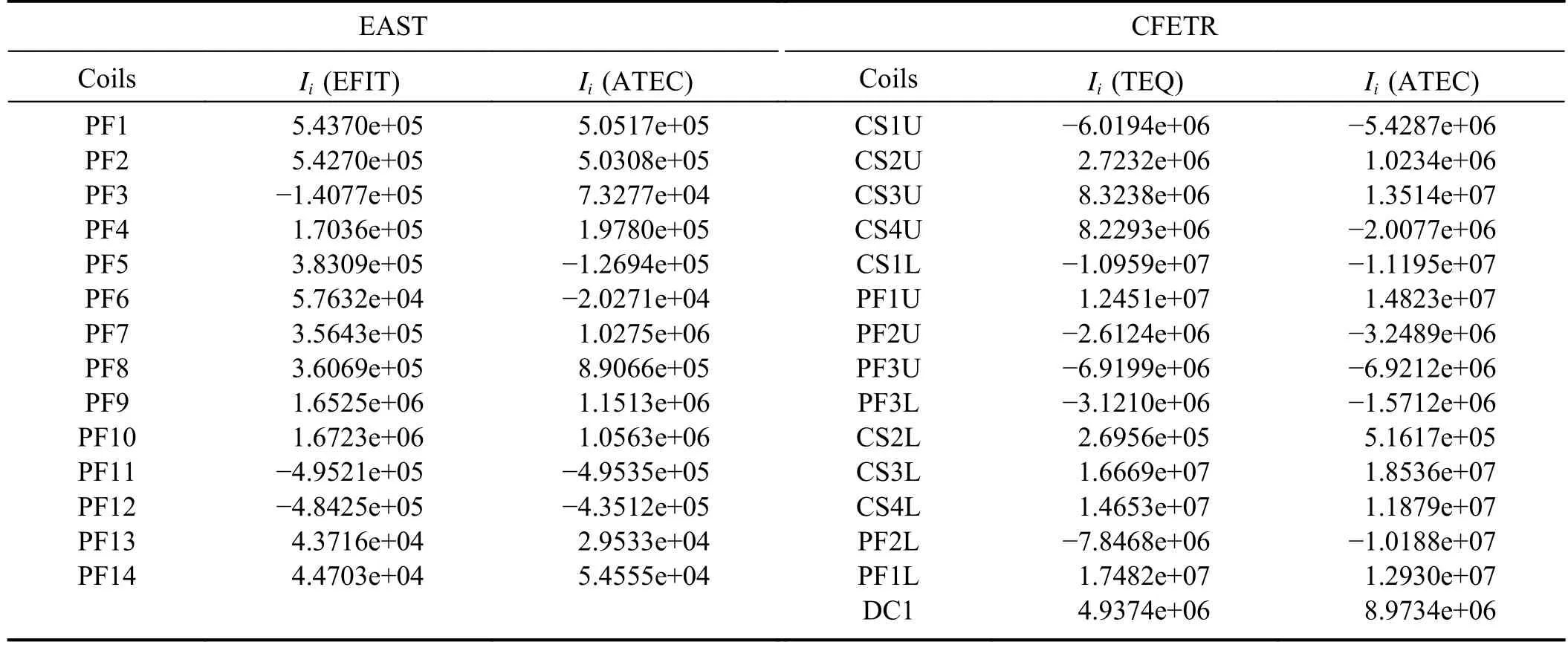
Table 1.Comparison of the coil current calculated by the three codes for EAST and CFETR (the unit of Ii is A).PF represents the poloidal field coil,CS represents the central solenoid coil,and DC represents the divertor-configuration coil.

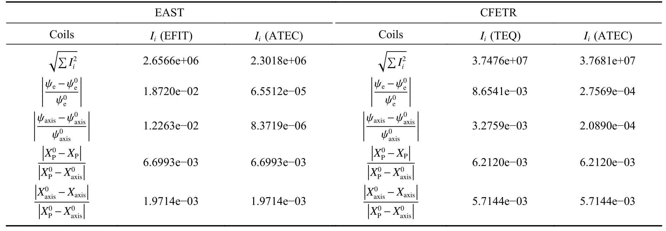
Table 2.Comparison of the total coil current,and the error of the LCFS calculated by the three codes for EAST and CFETR (the unit of Ii is A).X is the position vector.Here superscript 0 and without superscript represent the results of EFIT/TEQ and ATEC,respectively.The subscripts P,e ,and axis represent the X-point,boundary,and magnetic axis,respectively.

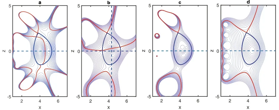
Figure 3.The figures (a),(b),(c) and (d) represent the HL-CREC,UD-CREC,C-CREC,and NEC,respectively.The fixed total plasma current Ip=0 for the HL-CREC,UD-CREC,Ip=-6e +05 A ,Ip/Ipin=-6 for the C-CREC and Ip=6e+ 05 A for the NEC,where Ipin is the prescribed negative current in the center subdomain of the plasma.The blue solid lines are the desired LCFSs of the plasma,and the red lines are the LCFSs of our numerical results.The horizontal dashed lines are x with z=0 in figures (a)-(d),and the longitudinal dashed line is z=0 with x=x0 in figure (b).

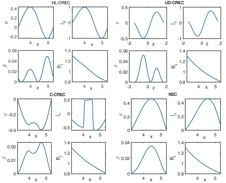
Figure 4.The profiles of ψ ,j? ,β,and Bt in the HL-CREC,C-CREC,and NEC change along x with z=0 in the plasma (the dashed lines in figures 3(a),(c),and (d)),respectively.The profiles of ψ ,j? ,and β in the UD-CREC change along z with x=x0 in the plasma,and Bt change along x with z=0 (the dashed lines in figure 3(b))

Table 3.Comparison of the coil currents,the total coil current and βp= calculated by ATEC for CRECs in EAST plasma.

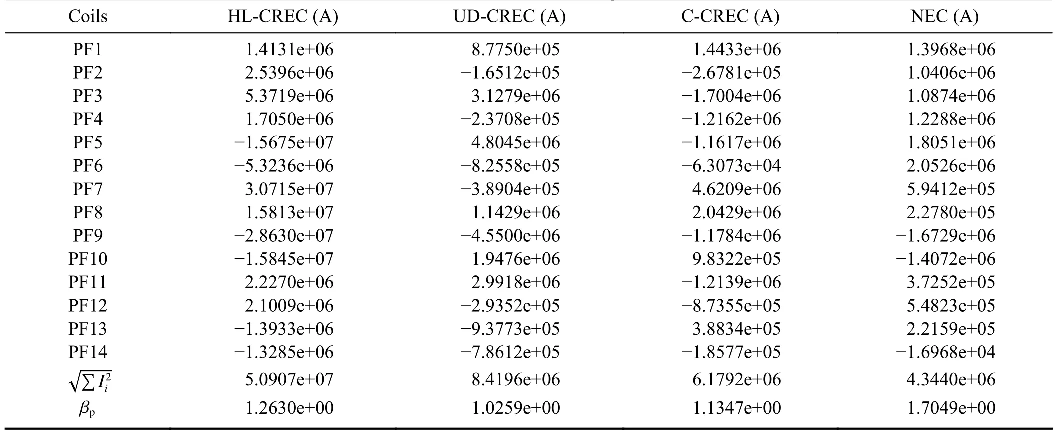
Table 3.Comparison of the coil currents,the total coil current and βp= calculated by ATEC for CRECs in EAST plasma.

Coils HL-CREC (A) UD-CREC (A) C-CREC (A) NEC (A)PF1 1.4131e+06 8.7750e+05 1.4433e+06 1.3968e+06 PF2 2.5396e+06 -1.6512e+05 -2.6781e+05 1.0406e+06 PF3 5.3719e+06 3.1279e+06 -1.7004e+06 1.0874e+06 PF4 1.7050e+06 -2.3708e+05 -1.2162e+06 1.2288e+06 PF5 -1.5675e+07 4.8045e+06 -1.1617e+06 1.8051e+06 PF6 -5.3236e+06 -8.2558e+05 -6.3073e+04 2.0526e+06 PF7 3.0715e+07 -3.8904e+05 4.6209e+06 5.9412e+05 PF8 1.5813e+07 1.1429e+06 2.0429e+06 2.2780e+05 PF9 -2.8630e+07 -4.5500e+06 -1.1784e+06 -1.6729e+06 PF10 -1.5845e+07 1.9476e+06 9.8322e+05 -1.4072e+06 PF11 2.2270e+06 2.9918e+06 -1.2139e+06 3.7252e+05 PF12 2.1009e+06 -2.9352e+05 -8.7355e+05 5.4823e+05 PF13 -1.3933e+06 -9.3773e+05 3.8834e+05 2.2159e+05 PF14 -1.3285e+06 -7.8612e+05 -1.8577e+05 -1.6968e+04√∑I2 i 5.0907e+07 8.4196e+06 6.1792e+06 4.3440e+06 βp 1.2630e+00 1.0259e+00 1.1347e+00 1.7049e+00

Figure 5.The figures (a),(b) represent respectively the HL-CREC and UD-CREC under smaller control coil currents.

Table 4.Comparison of the single coil currents,the total coil current,and the “absolute current” calculated by ATEC for CRECs in EAST plasma.

4.Summary and conclusions

In summary,an advanced tokamak equilibrium calculation code ATEC is developed by using the improved von Hagenow method.This method can transform the free boundary problem into a series of fixed boundary problems,which greatly improves the efficiency of solving G-S equations under more general current profiles.This code can be used for numerical simulation of more general free boundary problems of tokamak plasmas including the current-hole and current-reversal equilibrium.The most critical plasma current zero-crossing equilibrium problem in the AC operation process is investigated using this code.The results show that the configuration control of zero plasma current equilibrium can be achieved under the condition in which the coil control current is of the same order as that of the normal plasma equilibrium.At the same time,the current reversal equilibrium configuration can maintain similar confinement efficiency and related plasma parameters as the conventional configuration under some appropriate current profile conditions.In AC operation mode,the code can provide useful basic numerical analysis tools for the optimization of the equilibrium control coil current,the design of divertor plates,stability analysis,transport research and so on.Therefore,it may lay an important foundation for the successful realization of advanced high-parameter and high-confinement-efficiency AC operation in the future.

Acknowledgments

One of the authors (Yemin Hu) would like to express his thanks to Dr.Jiale Chen,Dr.Hang Li,Dr.Yanlong Li,Dr.Yueheng Huang,and Dr.Zhengping Luo for their equilibrium data files and helpful discussions.The authors would also like to acknowledge the ShenMa High Performance Computing Cluster at the Institute of Plasma Physics,Chinese Academy of Sciences.This work was supported by National Natural Science Foundation of China (No.12075276),and also partly by the Comprehensive Research Facility for Fusion Technology Program of China (No.2018-000052-73-01-001228).